Video-based sub-meter localization
Smartphone GPS receivers typically encounter an error of 10-15 meters under an open sky, and over 100 meters in challenging places (e.g., urban canyons), making applications such as navigation for the visually impaired essentially impossible. In this project, we developed a video-based localization solution with sub-meter accuracy using a smartphone’s camera. Here, we address three key challenges faced in video-based localization on smartphones. (a) 3D model construction using standard techniques is not robust to the varieties of smartphone video, (b) due to resource constraints, 3D model size must be kept to a minimum, and (c) feature extraction, particularly for accurate image features, remains computationally very costly. Based on an extensive set of both indoor and outdoor videos, meticulously annotated with location ground truth, we demonstrate that our proposed techniques produce accurate models despite challenging video conditions and substantially reduce model size without sacrificing accuracy. We also demonstrate an optical flow based method to reduce the feature extraction effort required for accurate localization.
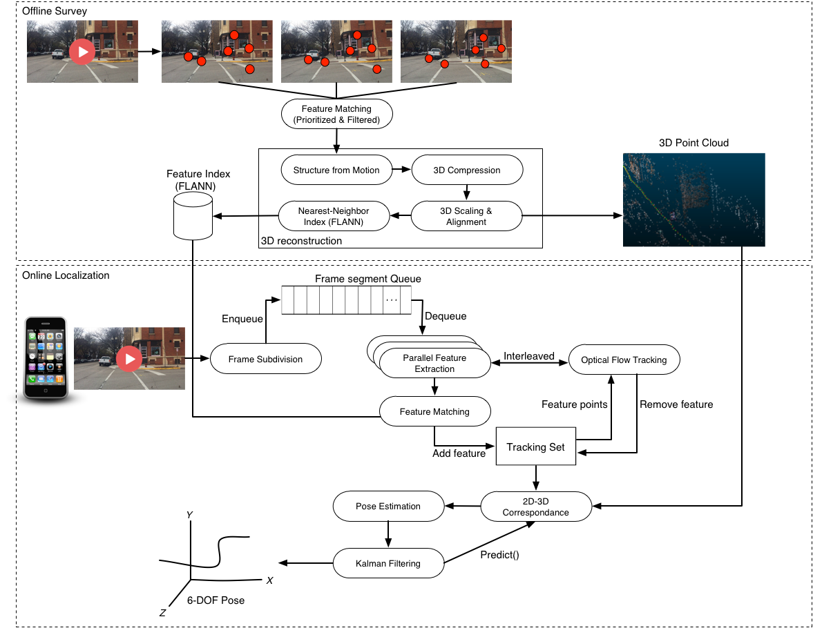
The figure below shows the pipelines for 3D environment reconstruction and localization.
We record a survey video in an area of interest and process it offline to reconstruct the 3D environment with compressed 3D point cloud and image features. During online localization, we use subdivided frame matching interleaved with optical flow tracking to estimate 6-DOF pose in near real time.
Additionally, we reduce the total 2D-3D correspondence by ordering them using projection error cutt-off obtained from Kalman filter predict() stage and sorted feature distances. This reduces both pose estimation time and optical flow tracking time in the next step. Finally, we use Kalman filter to correct the bad location estimation.
The video below shows an example of the reconstructed 3D point cloud of an urban street near UIC campus.
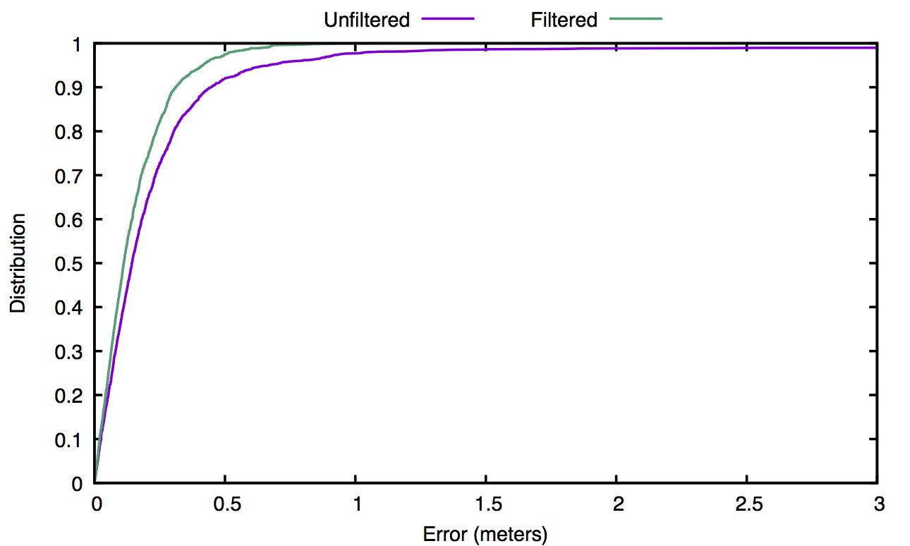
The plot below shows the CDF of both unfiltered and Kalman-filtered localization error. Here, the median error is under 0.2 meters.
Performance and cost optimization for online GPS tracking
For online GPS tracking of mobile devices, optimizing cellular data usage with a controllable error bound is an important problem. To investigate real world deployment, we studied a dataset consisting of 1.6 billion GPS points obtained from Nokia Research and found that 90% are sent using a naive periodic policy (1-300 second period). Through experiments we also found that every packet sent incurs significant overhead. Additionally, in online tracking, a fundamental three-way trade-off exists among timeliness, accuracy, and data usage. With these observations in mind, we designed a thrifty tracking system that allows the user to specify desired targets for any two of timeliness, accuracy, and cost; and optimizes the third. We also provided the first unified view of the three-way trade-off with a closed-form characterization equation.
The figure below shows the architecture of our online GPS tracking system. Starting in the top-left of the figure, a GPS receiver samples the (continuous) device location, often with a frequency of 1 Hz or higher. The incoming “raw” GPS trace (1) is first passed through a filter to remove any obvious outliers. An annotator then decorates each point with additional information not provided by the GPS receiver such as estimated velocity, acceleration, heading etc. Next, the decorated GPS trace (2) is passed to a sampler. The sampler unilaterally decides whether to forward a given trace point, with any necessary annotations, to the server. This decision is made based on one or more factors such as time, changes in speed, heading, recent data usage history, data usage budget or target, battery level, and perhaps most importantly extrapolation error, as discussed next. The resulting sampled trace (3) is then fed to two identical extrapolators: one running on the server, and one running on the mobile device. An extrapolator takes a sampled trace and an extrapolation database as input, and produces a continuous location estimate at the current time. On the server side, the extrapolator output (4) is made available for use by the trace consumer. On the client side, an identical extrapolator produces a continuous location estimate for local use in computing the current extrapolation error. This is provided as feedback to error-aware samplers. By comparing the output of the local extrapolator against the incoming raw GPS location, an error-aware sampler makes its forwarding decision based on the difference between the current estimate and the location reported by the GPS.
![]()
The video below shows the convergence of mean location error, mean data usage, and mean reporting delay representing the three-way trade-off among these three parameters.
See more at our TMC 2016 and GIS 2013 papers.
Passive localization and tracking using Wi-Fi
All smartphones come with Wi-Fi, and to detect the availability of Wi-Fi networks these smartphones periodically transmit probe messages. By deploying Wi-Fi monitors in an area of interest, it is possible to detect these transmissions, providing a coarse-grained location trace for each phone. Inspired by these observations, we developed a system to track unmodified smartphones, which enables applications such as monitoring street traffic flow. However, some major challenges for passive smartphone tracking are sparse packet transmissions, received signal strength variation, and a variable number of received packets. To address these challenges we used a hidden-Markov-model based solution, using map topology to impose restrictions on movement, and signal strength characteristics. Additionally, to obtain more packets from a passing smartphone for improved tracking accuracy, we used low-level Wi-Fi protocol features involving association process and management frames that increased the number of received packets by up to 5 times.
The video below illustrates the performance of our tracking method with Wi-Fi monitors placed approximately 500 meters apart. The red car shows the tracked location and the green car shows the ground truth GPS location.
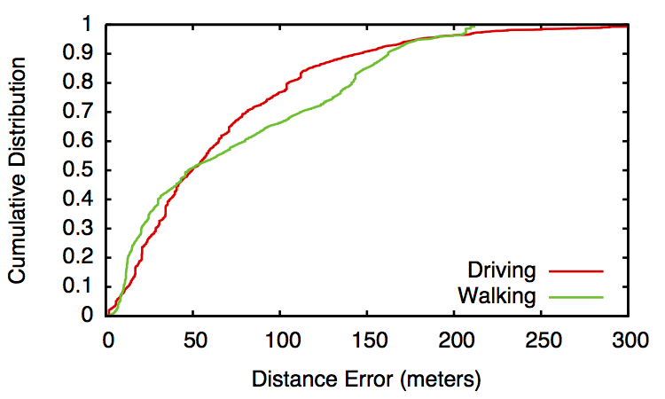
The figure below shows the CDF of tracking error for both driving and walking in the same setup as the above video. Here, the median error is 50 meters for both driving and walking.
See more at our SenSys 2012 paper and SenSys 2011 demo.
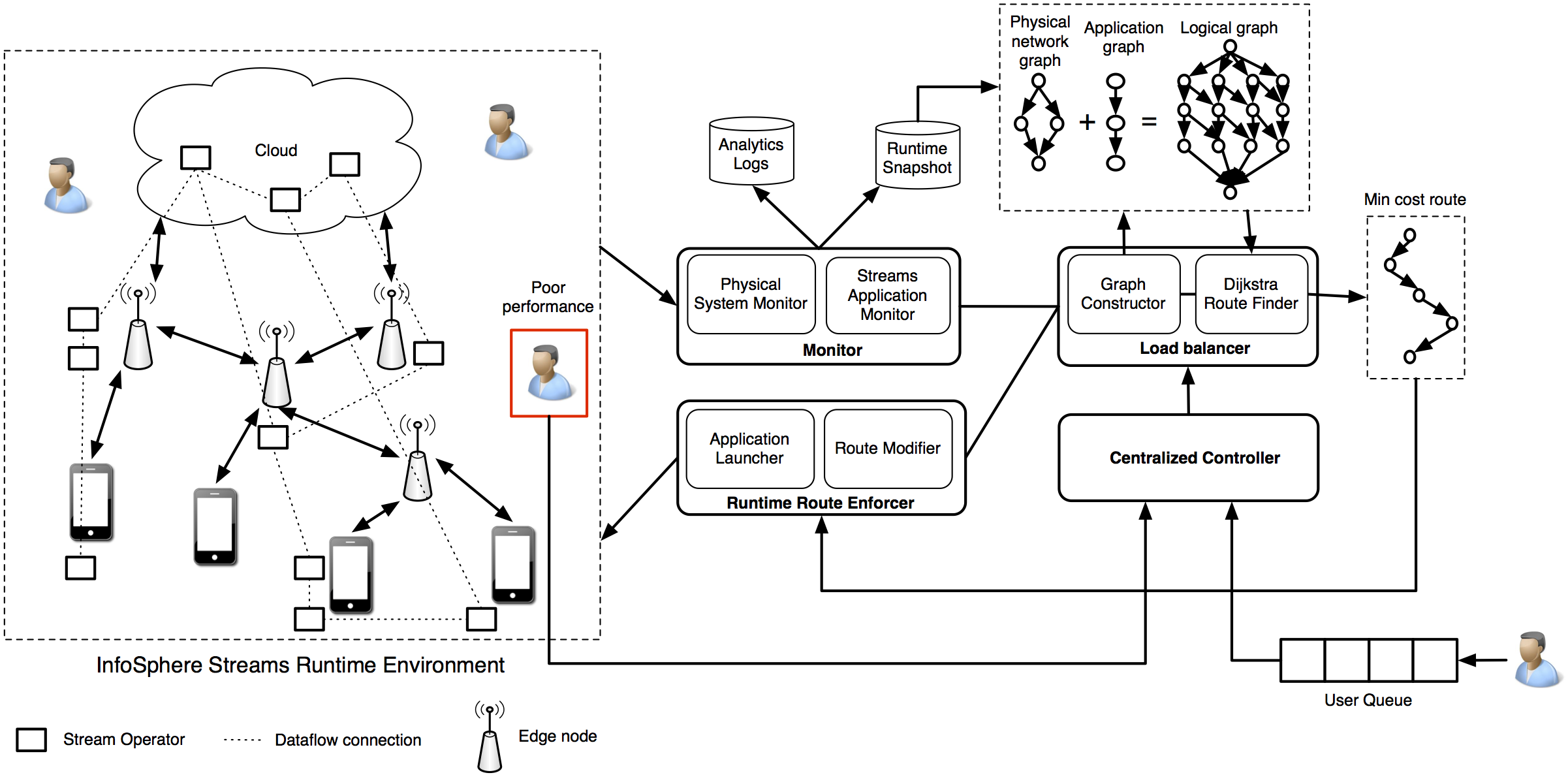
System architecture for data stream processing in mobile-edge-cloud architecture
Designing an efficient computational and network architecture is a challenge for real-time large-scale localization and tracking. Smartphones are not fast enough for many computational tasks (e.g., computer vision), and also constrained by limited battery power. To address these problems, in collaboration with IBM Research, we developed a framework for offloading computation to edge (e.g., servers connected over Wi-Fi or cellular access points) and cloud nodes. This framework distributes application computation across various processing nodes to achieve improved application performance and reduced latency.
The figure below shows the architecture of this system. Here, the stream data processing operators/jobs are deployed in mobile-edge-cloud nodes for many users simultaneously. We monitor both the physical resources (e.g., network latency and bandwidth, CPU and memory consumption) and application performance (e.g., frames-per-second, tuples-per-second) continuously. Hence the centralized controller can detect a poor-performing user and can attempt to load-balance the system. The centralized controller also controls the admission of new users from the user queue to guarantee a performance bound. The load balancer combines the physical network info with application info to form a logical graph. In this graph, the nodes are stream operator running at particular compute unit (mobile or edge or cloud) and the edges are connectivity between these operators. We model the edge costs as a function of affability of computing and network resource as well as the performance of the stream operators. Then, we apply Dijkstra’s shortest-path algorithm to find the optimal assignment of operators.