Smoothers

Regression is a statistical method that yields a most-likely value on a predicted variable y given a value of a predictor variable x. As Stephen Stigler describes, Francis Galton devised the method (and its name) to account for the relationship between parental and offspring traits. Since a hereditary trait relationship is not perfect (free of error), Galton sought a "most-probable" description of it.

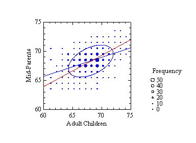
Galton used real data and a geometric drawing to derive his statistical model. The following figure contains a plot of his data (adapted from Stigler's table, typeset from the original table in Galton's paper cited below) and a fit of the model Galton devised. The vertical axis represents the average height of both parents of a child (Galton called this "mid-parent") and the horizontal axis represents the height of an adult child. The size of a symbol is proportional to the frequency of a pair of values in Galton's table. The ellipse in the figure is based on a bivariate normal distribution whose parameters have been estimated by SYSTAT from Galton's data. Galton inferred this ellipse (and its smaller and larger siblings) by linking similar values in his table of data, as we might link them by joining symbols of similar size. As Galton observed, the blue regression line passes through the two points where vertical lines are tangent to the ellipse (as well as through vertical-tangent points for any other member of this family of ellipses).

The red line is the major axis of the ellipse. It is a line we might instinctively draw if we were asked to predict parents' height from children's height. Notice, however, that the best-predicting (most-probable y value for a given x value) blue regression line pivots away from the red line and toward a horizontal line passing through mean parents' height (which Galton termed a line of "mediocrity"). We can perceive this effect in the figure by noting that the blue line passes near more large spots than does the red. This is the effect Galton called regression. He also observed that this effect was symmetric; it occurs when we predict x from y using this same model. Stigler shows how this observation influenced modeling in the social sciences for more than a century.

Galton's model requires us to assume bivariate normality in the population. Even if we relax that assumption, we are left with straight prediction lines. We could use polynomial models to allow curves, but modern statisticians have devised regression methods that allow the data to influence the shape of a prediction line instead of forcing us to decide on a model in advance. These methods are usually called nonparametric regression, or smoothing. Fan and Gijbels (1996) outline many of them.

The smoothing methods in this applet work by computing predictions from subsets of the data. A point (x, ypredicted) on the smooth is computed from a subset of data values (xi, yi), where the xi are the k nearest data neighbors of x (the method used in this applet) or within a chosen distance from x. There are two ways to compute the smoothed value on this subset of the data. Kernel methods (Mean and Median in this applet) compute a weighted average or simple order statistic of the data values. The weighting function for this kernel (Epanechnikov in this applet) usually favors the xi in the subset that are nearest to x, the predictor value. Polynomial methods (Polynomial and Loess in this applet) compute a linear or polynomial regression on the data values.

The buttons at the bottom of the applet control the size of the subsets used to compute each predicted point on the line. The default setting is half the data values. If you reduce the size (<), the curve gets wigglier and local and if you increase it (>), the curve gets more global. Use the Sample button at the top to pick new random samples.

There are a few things to learn from this applet. First, notice that the kernel methods tend to regress (toward Galton's "mediocrity") more at the endpoints of the smooth than do the polynomial methods. This is usually regarded as a flaw, although there are some unusual situations where you might want regressive predictions at extremes (did you lose money on high-flying dot.coms?). Second, compare Loess to Polynomial for several samples. I have programmed the generator to include occasional outliers. Notice that Loess is less influenced by these outliers. This is because William Cleveland designed Loess to include robust polynomial fitting, which down-weights data points with large residuals.

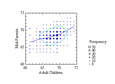
What would Galton have done with these techniques? From Stigler's description, I would guess that he would have been fascinated with them because he was a practical man interested as much in data as in models. The following figure shows a Loess smoother on Galton's data. I have also fit a kernel density contour to correspond to the ellipse in the figure above. There is a suggestion of greater regression for short families than for tall (a "kink" in the middle of the smooth), and the joint density isn't quite elliptical. Galton assumed that height was normally distributed, the result of small contributions from numerous, independent factors. This assumption served psychologists and geneticists well for almost a hundred years. Many researchers are now finding the normality assumption for traits to be an oversimplification.

To investigate the smoother kink a bit further, I fit the following linear model to the data:

where indicator is 1 if child>68 and 0 otherwise. I chose 68 inches because it is close to the mean for the child data. The t-statistic for the estimate of b2 has an associated probability of .00072. Where did this kink come from? There are numerous published citations of this dataset and several tutorials referring to it on the Web (you can find many by doing a Google search on the terms "Galton" and "regression"). I have not seen any sources that noticed this artifact, if indeed that is what it is.

Some of the discussions of Galton's discovery confuse the dataset in Galton's original paper with the datasets in Karl Pearson and Alice Lee's later papers. Galton did not plot height of fathers against height of sons. To support his argument, Galton averaged the parent data within families. He also shifted the female data upward by a constant to make them overlap with the male data in a single "pseudo-distribution." Pearson and Lee tabulated the data separately for fathers, mothers, sons, and daughters. I investigated whether Galton's kink could be reproduced by averaging the Pearson and Lee data and shifting the females by a constant. The kink did not appear.

I think that Galton's averaging and shifting blended two distributions (male and female) with different variances and covariances. Under certain circumstances, a kink could appear when a piecewise regression model is fit to data blended this way. Jerry Dallal believes that there is a common source underlying the data in the cited papers. Without access to the raw data, however, it is impossible to average within families.

I assigned this problem to Amanda Wachsmuth, a graduate student in my Northwestern graphics course last year. She investigated the Pearson and Lee data further and we think we have the answer. See "Galton's Bend" in the publications on the home page. It will be published in the August issue of The American Statistician.

Fan, J., and Gijbels, I. (1996). Local Polynomial Modelling and Its Applications. London: Chapman & Hall.

Galton, F. (1886). Regression Towards Mediocrity in Hereditary Stature, Journal of the Anthropological Institute of Great Britain and Ireland, 15, 246-263.

Pearson, K. and Lee, A. (1896). Mathematical Contributions to the Theory of Evolution. On Telegony in Man, &c., Proceedings of the Royal Society of London, 60, 273-283.

Pearson, K. and Lee, A. (1903). On the Laws of Inheritance in Man: I. Inheritance of Physical Characters, Biometrika, 2(4), 357-462.

Stigler, S. (1986). The History of Statistics. Cambridge: Harvard University Press.