Title
References:
- Andy Johnson's CS 488 Course Notes, Lecture XX
- Foley, Van Dam, Feiner, and Hughes, "Computer Graphics
- Principles and Practice", Chapter XX
Last time we talked about 3D projections from the theoretical point of view.
Today we are going to talk about how we actually implement the viewing of a 3D world on a 2D screen.
This involves a progression of transformations.
3D World -> Normalize to the canonical view volume -> Clip against canonical view volume -> Project onto projection plane -> Translate into viewport.
Again we want to come up with a matrix or set of matrices that we can repeatedly apply to all of the points in the 3D world to put them in their proper place in the 2D window on the computer screen.
Now, how do we actually IMPLEMENT this?!?!?!?
Here is where the matrices really start to go out of control. What is important to keep track of is the order in which things are performed, and not to get lost in the multitides of matrices.
There are 2 general ways to do this with the main difference being whether clipping is performed in world coordinates or homogeneous coordinates (see p.233 in red book, p.279 in white book). The second way is more general.
Method 1:
- Extend 3D coordinates to homogeneous coordinates
- Apply Npar or Nper to normalize the homogeneous coordinates
- Divide by W to go back to 3D coordinates
- Clip in 3D against the appropriate view volume (parallel or perspective)
- Extend 3D coordinates to homogeneous coordinates
- Perform projection using either Mort or Mper (with d=1)
- Translate and Scale into device coordinates
- Divide by W to go to 2D coordinates
Method 2:
- Extend 3D coordinates to homogeneous coordinates
- Apply Npar or Nper' to normalize the homogeneous coordinates
- Clip in homogeneous coordinates
- Translate and Scale into device coordinates
- Divide by W to go to 2D coordinates
The First Two Steps are Common to Both Methods
1. Extend 3D coordinates to homogeneous coordinates
This is easy we just take (x, y, z) for every point and add a W=1 (x, y, z, 1)
As we did previously, we are going to use homogeneous coordinates to make it easy to compose multiple matrices.
2. Normalizing the homogeneous coordinates
It is hard to clip against any view volume the user can come up with, so first we normalize the homogeneous coordinates so we can clip against a known (easy) view volume (the canonical view volumes).
That is, we are choosing a canonical view volume and we will manipulate the world so that the parts of the world that are in the existing view volume are in the new canonical view volume.
This also allows easier projection into 2D.
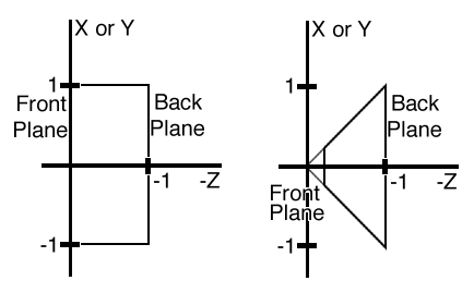
In the parallel projection case the volume is defined by these 6 planes:
x = -1    y = -1    z = 0
x = 1     y = 1     z = -1
In the perspective projection case the volume is defined by these 6 planes:
x = -z    y = -z    z = -zmin
x =  z    y =  z    z = -1
We want to create Npar and Nper, matrices to perform this normalization.
For Npar the steps involved are:
- Translate VRP to the origin
- Rotate VRC so n-axis (VPN) is z-axis, u-axis is x-axis, and v-axis is y-axis
- Shear so direction of projection is parallel to z-axis (only needed for oblique parallel projections - that is where the direction of projection is not normal to the view plane)
- Translate and Scale into canonical view volume
Step 2.1 Translate VRP to the origin is T(-VRP)
Step 2.2 Rotate VRC so n-axis (VPN) is z-axis, u-axis is x-axis, and v-axis is y-axis uses unit vectors from the 3 axis:
Rz = VPN / || VPN || (so Rz is a unit length vector in the direction of the VPN)
Rx = VUP x Rz / || VUP x Rz || (so Rx is a unit length vector perpendicular to Rz and Vup)
Ry = Rz x Rx (so Ry is a unit length vector perpendicular to the plane formed by Rz and Rx)
giving matrix R:
_                 _
| r1x  r2x  r3x  0 |
| r1y  r2y  r3y  0 |
| r1z  r2z  r3z  0 |
| 0    0    0    1 |
-                 -
with rab being the ath element of Rb
VPN rotated into Z axis, U rotated into X, V rotated into Y
now the PRP is in world coordinates
Step 2.3 Shear so direction of projection is parallel to z-axis (only needed for oblique parallel projections - that is where the direction of projection is not normal to the view plane) makes DOP coincident with the z axis. Since the PRP is now in world coordinates we can say that:
DOP is now CW - PRP
_   _    _              _    _     _
|DOPx|   | (umax+umin)/2 |   | PRPu |
|DOPy| = | (vmax+vmin)/2 | - | PRPv |
|DOPz|   |      0        |   | PRPn |
| 0  |   |      1        |   |  1   |
-   -    -              -    -     -
We need DOP to be:
_    _
| 0   |
| 0   |
|DOPz'|
| 1   |
-    -
The shear is performed with the following matrix:
_             _
| 1  0  shx  0 |
| 0  1  shy  0 |
| 0  0    1  0 |
| 0  0    0  1 |
-             -
where:
shx = - DOPx / DOPz
shy = - DOPy / DOPz
note that if this is an orthographic projection (rather than an oblique one) DOPx = DOPy=0 so shx = shy = 0 and the shear matrix becomes the identity matrix.
*** note that the red book has 2 misprints in this section. Equation 6.18 should have dopx as the first element in the DOP vector, and equation 6.22 should have dopx / dopz. The white book has the correct versions of the formulas
Step 2.4 Translate and Scale the sheared volume into canonical view volume:
Tpar = T( -(umax+umin)/2, -(vmax+vmin)/2, -F)
Spar = S( 2/(umax-umin), 2/(vmax-vmin), 1/(F-B))
where F and B are the front and back distances for the view volume.
So, finally we have the following procedure for computing Npar:
Npar = Spar * TPar * SHpar * R * T(-VRP)
For Nper the steps involved are:
- Translate VRP to the origin
- Rotate VRC so n-axis (VPN) is z-axis, u-axis is x-axis, and v-axis is y-axis
- Translate so that the center of projection(PRP) is at the origin
- Shear so the center line of the view volume is the z-axis
- Scale into canonical view volume
Step 2.1 Translate VRP to the origin is the same as step 2.1 for Npar: T(-VRP)
Step 2.2 Rotate VRC so n-axis (VPN) is z-axis, u-axis is x-axis, and v-axis is y-axis is the same as step 2.2 for Npar:
Step 2.3 Translate PRP to the origin which is T(-PRP)
Step 2.4 is the same as step 2.3 for Npar. The PRP is now at the origin but the CW may not be on the Z axis. If it isn't then we need to shear to put the CW onto the Z axis.
Step 2.5 scales into the canonical view volume
up until step 2.3, the VRP was at the origin, afterwards it may not be. The new location of the VRP is:
                         _  _
                         | 0 |
VRP' = SHpar * T(-PRP) * | 0 |
                         | 0 |
                         | 1 |
                         -  -
so
Sper = ( 2VRP'z / [(umax-umin)(VRP'z+B)] , 2VRP'z / [(vmax-vmin)(VRP'z+B)], -1 / (VRP'z+B))
So, finally we have the following procedure for computing Nper:
Nper = Sper * SHpar * T(-PRP) * R * T(-VRP)
You should note that in both these cases, with Npar and Nper, the matrix depends only on the camera parameters, so if the camera parameters do not change, these matrices do not need to be recomputed. Conversely if there is constant change in the camera, these matrices will need to be constantly recreated.
The Remaining Steps Differ for the Two Methods
Now, here is where the 2 methods diverge with method one going back to 3D coordinates to clip while method 2 remains in homogeneous coordinates.
The choice is based on whether W is ensured to be > 0. If so method 1 can be used, otherwise method 2 must be used. With what we have discussed in this class so far W will be > 0, and W should remain 1 thorought the normaliztion step. You get W < 0 when you do fancy stuff like b-splines. Method 2 also has the advantage of treating parallel and perspective cases with the same clipping algorithms, and is generally supported in modern hardware.
We will deal with Method 1 first.
3. Divide by W to go back to 3D coordinates
This is easy we just take (x, y, z, W) and divide all the terms by W to get (x/W, y/W, z/W, 1) and then we ignore the 1 to go back to 3D coordinates. We probably do not even need to divide by W as it should still be 1.
4. Clip in 3D against the appropriate view volume
At this point we want to keep everything that is inside the canonical view volume, and clip away everything that is outside the canonical view volume.
We can take the Cohen-Sutherland algorithm we used in 2D and extend it to 3D, except now there are 6 bits instead of four.
For the parallel case the 6 bits are:
- point is above view volume: y > 1
- point is below view volume: y < -1
- point is right of view volume: x > 1
- point is left view volume: x < -1
- point is behind view volume: Z < -1
- point is in front of view volume: z > 0
For the perspective case the 6 bits are:
- point is above view volume: y > -z
- point is below view volume: y < z
- point is right of view volume: x > -z
- point is left view volume: x < z
- point is behind view volume: z < -1
- point is in front of view volume: z > zmin
P273 in the white book shows the appropriate equations for doing this.
5. Back to homogeneous coordinates again
This is easy we just take (x, y, z) and add a W=1 (x, y, z, 1)
6.Perform Projection - Collapse 3D onto 2D
For the parallel case the projection plane is normal to the z-axis at z=0. For the perspective case the projection plane is normal to the z axis at z=d. In this case we set z = -1.
In the parallel case, since there is no forced perspective, Xp = X and Yp = Y and Z is set to 0 to do the projection onto the projection plane. Points that are further away in Z still retain the same X and Y values - those values do not change with distance.
For the parallel case, Mort is:
_            _
| 1  0  0  0 |
| 0  1  0  0 |
| 0  0  0  0 |
| 0  0  0  1 |
-            -
Multiplying the Mper matrix and the vector (X, Y, Z, 1) holding a given point, gives the resulting vector (X, Y, 0, 1).
In the perspective case where there is forced perspective, the projected X and Y values do depend on the Z value. Objects that are further away should appear smaller than similar objects that are closer.
For the perspective case, Mper is:
_            _
| 1  0  0  0 |
| 0  1  0  0 |
| 0  0  1  0 |
| 0  0 -1  0 |
-            -
Multiplying the Mper matrix and the vector (X, Y, Z, 1) holding a given point, gives the resulting vector (X, Y, Z, -Z).
7. Translate and Scale into device coordinates
All of the points that were in the original view volume are still within the following range:
-1 <= X <= 1
-1 <= Y <= 1
-1 <= Z <= 0
In the parallel case all of the points are at their correct X and Y locations on the Z=0 plane. In the perspective case the points are scattered in the space, but each has a W value of -Z which will map each (X, Y, Z) point to the appropriate (X', Y') place on the projection plane.
Now we will map these points into the viewport by moving to device coordinates.
This involves the following steps:
- translate view volume so its corner (-1, -1, -1) is at the origin
- scale to match the size of the 3D viewport (which keeps the corner at the origin)
- translate the origin to the lower left hand corner of the viewport
Mvv3dv = T(Xviewmin, Yviewmin, Zviewmin) * Svv3dv * T(1, 1, 1)
where
Svv3dv = S( (Xviewmax-Xviewmin)/2, (Yviewmax-Yviewmin)/2, (Zviewmax-Zviewmin)/1 )
You should note here that these parameters will only depend on the size and shape of the viewport - they are independant of the camera settings, so if the viewport is not resized, these matrices will remain constant and reusable.
*** note that the red book has another misprint in this section. The discussion of the translation matrix before equation 6.44 has a spurious not equal to sign.
8. Divide by W to go from homogeneous to 2D coordinates
Again we just take (x, y, z, W) and divide all the terms by W to get (x/W, y/W, z/W, 1) and then we ignore the 1 to go back to 3D coordinates.
In the parallel case dropping the W takes us back to 3D coordinates with Z=0, which really means we now have 2D coordinates on the projection plane.
In the perspective projection case, dividing by W will affect the transformation of the points. Dividing by W (which is -Z) takes us back to the 3D coordinates of (-X/Z, -Y/Z, -1, 1). Dropping the W takes us to the 3D coordinates of (-X/Z, -Y/Z, -1) which positions all of the points onto the Z=-1 projection plane which is what we wanted. Dropping the Z coordinate gives us the 2D location on the Z=-1 plane.
The Second Method
BUT ... there is still the second method where we clip in homogeneous coordinates to be more general
The normalization step (step 2) is slighly different here, as both the parallel and perspective projections need to be normalized into the canonical parallel perspective view volume.
Npar above does this for the parallel case.
Nper' for the perspective case is M * Nper. Nper is the normalization given in step 2. This is the same normalization that needed to be done in step 8 of method one before we could convert to 2D coordinates.
M =
| 1 |
0 |
0 |
0 |
| 0 |
1 |
0 |
0 |
| 0 |
0 |
1/(1+Zmin) |
z/(1+Zmin) |
| 0 |
0 |
-1 |
0 |
Now in both the parallel and perspective cases the clipping routine is the same.
Again we have 6 planes to clip against:
- X = -W
- X = W
- Y = -W
- Y = W
- Z = -W
- Z = 0
but since W can be positive or negative the region defined by those planes is different depending on W.
2nd method step 4: Then we know all of the points that were in the original view volume are now within the following range:
-1 <= X <= 1
-1 <= Y <= 1
-1 <= Z <= 0
Now we need to map these points into the viewport by moving to the device coordinates.
This involves the following steps:
- translate view volume so its corner (-1, -1, -1) is at the origin
- scale to match the size of the 3D viewport (which keeps the corner at the origin)
- translate the origin to the lower left hand corner of the viewport
Mvv3dv = T(Xviewmin, Yviewmin, Zviewmin) * Svv3dv * T(1, 1, 1)
where
Svv3dv = S( (Xviewmax-Xviewmin)/2, (Yviewmax-Yviewmin)/2, (Zviewmax-Zview.min)/1 )
The new x and new y give us the information we need for the 2D version, but we will also find the new z to be useful for determining occlusion - which we will discuss in a few weeks as z-buffer techniques.
2nd method step 5: Then we divide by W to go from homogeneous to 2D coordinates. In the perspective projection case, dividing by W will affect the transformation of the points.
*** note that the red book has another misprint in this section. The discussion of the translation matrix before equation 6.44 has a spurious not equal to sign.