Resources

Throughout the semester, I will fill this webpage with useful resources. Most (if not all) of these resources will be freely available online.

Lecture Notes

For the few times I give lectures in class, I will post lecture notes here, along with other relevant materials.

Lecture 10 (Sept. 24, 2026) Notes from LeetCode Problem 105

We began this lecture by re-visiting the problem given in Lecture 9 (see below). Associated in-class drawings can be found here.

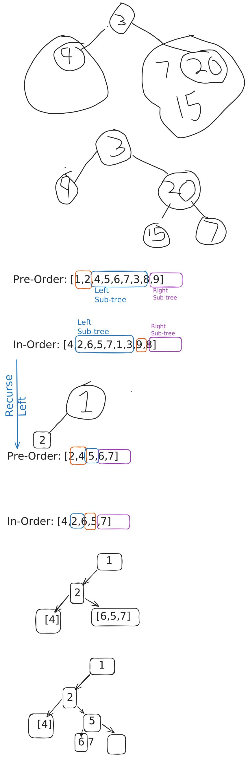
You are given two lists L1 and L2 of the same size. L1 represents the preorder traversal of a binary tree, and L2 is the inorder traversal. From this information, you are tasked with reconstructing the actual binary tree as a TreeNode data structure.

The high-level idea is simple for this problem. Given the root of a binary tree root, a preorder traversal does the following:

1. visits root,
2. recursively visits the left subtree root.left, and
3. recursively visits the right subtree root.right.

Note here that “visits” is a catch-all term for “do something at this tree node”. By definition, all null or nil nodes are visited.

Then, given root, an inorder traversal does the following:

1. recursively visits the left subtree root.left, and
2. visits root,
3. recursively visits the right subtree root.right.

From this, the algorithm for the specified problem is easy to state at a high level.

1. L1[0] is the root of the binary tree.

2. Search L2 for index i such that L1[0] == L2[i].

3. Now, from the definition of inorder traversal, we know that L2[:i] (note here i is exclusive, so this is L2[0], ..., L2[i-1]) are all nodes that appear in the left subtree of the binary tree rooted at L1[0], and L2[i+1:] are all nodes that appear in the right subtree of the binary tree rooted at L1[0].

4. Let l = len(L2[:i]) and r = len(L2[i+1:]). Then, we know that:

   • L1[1:l+1] is the preorder traversal of the left subtree of the binary tree rooted at L1[0], and
   • L1[l+1:] is the preorder traversal of the right subtree of the binary tree rooted at L1[0].

5. From here, we can recurse on the left subtree with preorder list L1[1:l+1] and inorder list L2[:i+1], and the right subtree with preorder list L1[l+1:] and inorder list L2[i+1:].

Lecture 7 (Sept. 15, 2026) Binary Trees and Merkle Trees

In this lecture, I tried to give some insight behind Merkle Trees, which you are asked to implement for your Project 2. Handwritten notes can be found here.

Review: Binary Trees

In general, trees are one of the most important data structures in computer science; they are used everywhere. Here, we focus on Binary trees, which are trees such that every node has at most 2 children.

Suppose we have the following TreeNode data structure to represent a binary tree.

struct TreeNode {
    // three basic things you'd want in a TreeNode
    string node_id; // this can also be an integer/char/short/a custom datatype/etc.
    TreeNode* left_child;
    TreeNode* right_child;
    // may contain other useful data
    // ...
}

Clearly from the above, trees are recursively defined data structures: a tree is either a leaf node, which has no children (i.e., left_child == right_child == null), or it is a rooted tree root which has two subtrees: a left subtree with root left_child and a right subtree with root right_child. Thinking about trees as recursive data structures greatly helps with understanding a variety of algorithms which use trees.

Traversing Trees. One of the most basic things you’d like to do when given a tree (besides trying to build a tree) is to perform some type of tree traversal: go through and “visit” every node in the tree. Here, “visiting” a node can mean a variety of things, including:

• Print node_id;
• Mark the node as visited; e.g., modify the struct TreeNode to include a boolean visited variable initially set to false.
• Update some node_distance value;
• etc.

Intuitively, “visiting” a node is a catch-all term for “do something at this node in the tree”. Now, the important question in any traversal is: what order do you visit each node in the tree?

Pre-order Traversal. A pre-order traversal is one of several types of depth-first traversals. You can think of these as recursive traversals. Intuitively, a pre-order traversal:

1. Begins at the root of the tree and immediately visits the root,
2. Then, the traversal recurses on the left subtree (i.e., go back to (1) above, but treat the left child as the new root to visit), followed by the right subtree.

As pseudocode, this traversal is done as follows.

void pre_order(TreeNode* root) {
    if(root == null) return;
    visit(root); // e.g., std::cout << root->node_id << std::endl;
    pre_order(root->left_child);
    pre_order(root->right_child);
}

Again, it is helpful to think about trees as recursive data structures: a pre-order traversal visits the root of a tree, then recurses on the left subtree (which has its own root), and on the right subtree (which also has its own root). The base case is either a leaf node (no children), or a null node (which is handled in the above pseudocode).

An example tree is given below.

graph TB
    a((a))-->b((b))
    a-->c((c))
    b-->d((d))
    b-->e((e))
    c-->f((f))
    c-->g((g))

The pre-order traversal of the tree would then be [a, b, d, e, c, f, g].

Post-order Traversal. Post-order traversal is essentially the reverse of a pre-order traversal. Again, thinking recursively: from the root of a tree,

1. Traverse the left subtree;
2. Traverse the right subtree;
3. Visit the root (i.e., the root is only visited after all nodes in the left and right subtrees are visited)

Now, as pseudocode, this traversal is done as follows.

void post_order(TreeNode* root) {
    if(root == null) return;
    post_order(root->left_child);
    post_order(root->right_child);
    visit(root); // e.g., std::cout << root->node_id << std::endl;
}

The post-order traversal of the previous tree would then be [d, e, b, f, g, c, a].

Back to Merkle Trees

This digression to trees and tree traversals was meant to get you thinking about trees so you can get some intuition behind Merkle Trees. A Merkle tree is an implicitly defined complete binary tree: given a list of $2^n$ node_id’s, a Merkle tree asks you to label a complete binary tree¹ as follows. Let vector<string> L be a list/vector of size $2^n$, and let H be a hash function which hashes strings to strings.

1. For each i in range(len(L)): leaf node i has label H( L[i] + "i"), where + denotes string concatenation, and "i" denotes converting integer i into a string.
2. For each non-leaf node v, label v as H( v.left_child.node_id + v.right_child.node_id ).

The final output of the Merkle tree commitment is the label of the root node in this complete binary tree. Now, this is a bit of a different tree problem you are given: the complete binary tree is only implicitly defined with respect to the input list L. However, from this list, you can label every node in a complete binary tree whose leaf nodes all have node_id = H( L[i] + "i" ).

Thinking in terms of tree traversals, imagine for a moment that you are given the root of this complete binary tree, and that all the leaf labels were given to you. Then, the output of a Merkle tree commitment is the root label after you’ve done a post_order labeling of the tree!

Given as pseudocode, this traversal is done as follows.

void post_order_label(TreeNode* root, HashFunction H) {
    // Assumption is that the leaves are already labeled.
    if(root->left_child == null && root->right_child == null) return; 
    post_order_label(root->left_child, H);
    post_order_label(root->right_child, H);
    root->node_id = H( root->left_child->node_id + root->right_child->node_id);
}

Suppose that you have TreeNode* myRoot as your root node. Then, you can run post_order_label(myRoot, H), and then the Merkle tree commitment simply outputs myRoot->node_id.

The key challenge with a Merkle tree is that you are not given myRoot! You are instead given the list L, which tells you how to label the leaf nodes in the above algorithm. From L and H, you can still recover myRoot->node_id if you were given myRoot instead.

Merkle Proofs. The amazing feature of a Merkle tree is that once you give someone the value of myRoot->node_id, they can later ask the following question: “What is item 5 in your list L?” Of course, if you trust the person who created the Merkle tree, they can reply with “Item 5 is L[5]”, and you both move on with your days. However, Merkle trees are used in situations where you do not trust the person who gave you myRoot->node_id! For example, they may be malicious and give you some other value instead of L[5] used in computing myRoot->node_id.

So then, you ask instead the question: “What is item 5 in your list L? Can you prove that your answer is consistent/agrees with the value myRoot->node_id which you gave me earlier?” This is a lot of words to say that a Merkle tree allows you to prove the authenticity of your data, and that it is consistent with the value myRoot->node_id you computed earlier.

As an example, suppose you begin with the list L = ['a', 'b', 'c', 'd']. First, let’s compute the Merkle tree below.

graph TB
    0(("('a',0)"))-->a
    1(("('b',1)"))-->b
    2(("('c',2)"))-->c
    3(("('d',3)"))-->d
    a(("h_a0 = H('a0')"))
    b(("h_b1 = H('b1')"))
    c(("h_c2 = H('c2')"))
    d(("h_d3 = H('d3')"))
    a-->e(("h_ab = H( h_a0+h_b1  )"))
    b-->e 
    c-->f(("h_cd = H( h_c2+h_d3 )"))
    d-->f
    e-->g(("h_abcd = H( h_ab+h_cd )"))
    f-->g
    linkStyle default stroke-width:2pt;

The output of the Merkle commitment would be h_abcd, the root label of the above tree.

Suppose you are given the string h_abcd, the output of the root label from the above tree. Now, in the Merkle proof, let’s say you ask for index i = 2. We provide the value L[2] = 'c', and now we also need to provide additional values to the proof so that you can verify ('c', 2) is consistent with h_abcd. Let proof = [] denote the proof string. We first have proof.append(L[2]), which gives us proof = [ 'c' ].

Now, intuitively, the proof proof needs to contain the minimum amount of information you need to compute h_abcd given you have h_abcd and you have information c and i=2. How do you figure out this information? Well, in the above tree, let’s highlight in red the root-to-leaf path from h_abcd to node ('c',2), given below as a red path.

graph TB
    0(("('a',0)"))-->a
    1(("('b',1)"))-->b
    2(("('c',2)"))-->c
    3(("('d',3)"))-->d
    a(("h_a0 = H('a0')"))
    b(("h_b1 = H('b1')"))
    c(("h_c2 = H('c2')"))
    d(("h_d3 = H('d3')"))
    a-->e(("h_ab = H( h_a0+h_b1  )"))
    b-->e 
    c-->f(("h_cd = H( h_c2+h_d3 )"))
    d-->f
    e-->g(("h_abcd = H( h_ab+h_cd )"))
    f-->g
    linkStyle default stroke-width:2pt;
    linkStyle 2 stroke:red,stroke-width:3pt;
    linkStyle 6 stroke:red,stroke-width:3pt;
    linkStyle 9 stroke:red,stroke-width:3pt;

Notice that given ('c',2), you can compute h_c2 as H=('c2'). Next, you must be able to compute h_cd. You can compute h_c2, but you cannot compute h_d3! So, instead, we ask the creator of the Merkle tree to give us this value in the proof. Notice that if you have h_d3, then you can compute h_cd = H(h_c2 + h_d3)! So proof.append(h_d3), and now the proof is proof = ['c', h_d3].

Now, with the proof so far, you can compute h_cd, but you cannot compute h_ab! And without h_ab, you cannot compute h_abcd, which is supposed to be the label of the root in the Merkle tree. So again, we ask the creator of the Merkle tree to give us h_ab so we can compute this value! Thus, we have proof.append(h_ab), and the final proof is proof = ['c', h_d3, h_ab]

You now have all the information needed to check if ('c', 2) is consistent with h_abcd. You compute h_c2 = H('c2'), then compute h_cd = H( h_cd + proof[1]), and finally check if h_abcd == H( proof[2] + h_cd). Done!

Lecture 6 (Sept. 10, 2026) Birthday Attacks

In this lecture, we discussed finding collisions in a hash function using something called a Birthday Attack, named after the Birthday Paradox.

In principle, a hash function $H$ is a compressing map from arbitrary-length strings, represented as ${{0,1}^{$}}\vphantom{}, to fixed-length strings. For positive integer $\lambda$, a hash function is a map $H \colon {0,1}^* \rightarrow {0,1}^\lambda$. It takes any binary string as input and outputs some binary string of length $\lambda$. Usually, we only think about hash functions with fixed-length inputs, such as $H : {0,1}^{2\lambda} \rightarrow {0,1}^\lambda$, which maps bit-strings of length $2\lambda$ to bit-strings of length $\lambda$ (it is a 2-to-1 compressing map).

Ideally, it should be very difficult to find collisions in a hash function. That is, finding two inputs $a \neq b$ such that $H(a) = H(b)$ should be hard. Indeed, if $H$ behaves like a random function, then the probability you find a collision is at most $\frac{1}{2^\lambda}$. However, $H$ is compressing, so collisions are guaranteed to exist by the Pigeonhole Principle.

Birthday Attacks

A birthday attack exploits the Birthday paradox to find collisions in a hash function. It is a very simple attack and works as follows.

1. Randomly choose $\sqrt{2^\lambda} = 2^{\lambda/2}$ inputs to the hash function. Let these inputs be named $x_1, \dotsc, x_{2^{\lambda/2}}$.
2. For each $i \neq j$, check if $H(x_{i}) = H(x_{j})$.

The above algorithm takes $O(2^{\lambda/2})$ time and space to execute. Note that step (2) above takes $O(2^\lambda)$ time if you check all possible pairs naively (e.g., you can use a hash-table to check if you have a collision!). Now, this is bad in practice, where $\lambda = 256$ is typical. This would be approximately $4 \times 10^{22}$ petabytes. Next lecture, we’ll see a much more space-efficient birthday attack algorithm.

More Reading and Resources

Additional reading can be found here: https://people.cs.uchicago.edu/~davidcash/284-autumn-21/12-hash.pdf. Calculator for the Birthday Problem found here: https://www.bdayprob.com/

Lecture 3 (Sept. 01, 2026) Counting Sort and Radix Sort

In this lecture, we learned about Counting Sort and Radix Sort. Handwritten notes can be found here.

Counting Sort

Suppose you are tasked with sorting integers in a given list $L$ of size $n$. Suppose further you are guaranteed that every integer $\ell \in L$ satisfies $0 \leq \ell \leq K$, where $K\geq 1$ is some positive integer. That is, everything in your dataset is guaranteed to be at least $0$ and at most the value $K$. Given this fact, can we sort $L$ in faster than $O(n\log(n))$ time?

All comparison-based sorts we saw in last lecture have a $\Omega(n \log(n))$ lower bound on their run time (specifically, the number of comparisons they make) when given any arbitrary list as input. In this problem, you are given a somewhat arbitrary list, but you have guarantees about the data set. We will use these guarantees to sort $L$ faster.

The simplest idea is to count how many times each element $\ell \in L$ occurs. Since you know that $0 \leq \ell \leq K$, we can sort the list as follows (using pseudocode).

def countingSort(L):
    # Allocates an array of size K+1 integers; we will use this to count.
    A = [ 0 for i in range(K+1) ] 
    for l in L:
        A[l] = A[l] + 1 # count how many times element l occurs in list L

    L.clear() # empty the list so we can use it again

    # add 0, 1, ..., K back to the list depending on the number of
    # times we saw it before
    for i in range(K+1): 
        # using the count we computed, add each element back to 
        # list L
        while size(A[i]) > 0:
            L.append(i) # append element i to L
            A[i] = A[i]-1 # decrement the count

    return L

The idea with counting sort above is to simply count the occurrence of each $\ell \in {0,1,\dotsc, K}$ that appear in the original list $L$. We use the array $A$ to track these occurrences. Once we have counted, we simply have to scan $A$ in order from index $0$ to index $K$, adding index $i$ exactly $A[i]$ times to the list $L$ (which we have cleared).

This algorithm runs in time $O(K + n)$, where $n$ is the size of your input list $L$ and $K$ is the upper bound on the values taken by your list $L$. The space is $O(K + n)$ as well. So long as $K = O(n)$, this algorithm works pretty well. However, it is quite likely that $K$ can be quite large when handling arbitrary data; for example, $K = 2^{32}-1$ for all possible unsigned integers, and you are allocating an array of size $2^{32}$, which can be quite large. This is even worse if $K = 2^{64}-1$ (unsigned integers), or if you need to handle larger integer types. Can we sort a list of $n$ integers in linear time without counting sort?

See also https://www.w3schools.com/dsa/dsa_algo_countingsort.php

Radix Sort

Radix sort essentially says “let’s use counting sort, digit by digit, for our integer inputs”. We will discuss LSB radix sort, which performs sorting in order from the least significant bit/digit to the most significant.

As an example, consider $L = [123, 52, 1677, 17]$. Scanning from the start to end of $L$, for each digit starting with the least significant, perform counting sort on those digits while preserving the original numbers. This means we have an array $A = [ [], …, [] ]$ of size $10$. Sorting by LSB, we see that $A[2] = [ 52 ]$, $A[3] = [ 123 ]$, and $A[7] = [1677, 17]$, with all other lists being empty. Now, we output a new list $L = [ 52, 123, 1677, 17 ]$, in sorted order of the LSB.

Continuing again to the second digits, we have $A[1] = [ 123, 17 ]$, $A[5] = [ 52 ]$, and $A[7] = [ 1677 ]$, and obtain the new sorted list $L = [ 123, 17, 52, 1677 ]$. With the third digits, we can write $017$ and $052$, and we get $A[0] = [ 17, 52 ]$, $A[1] = [ 123 ]$, and $A[6] = [1677]$, giving us $L = [17, 52, 123, 1677 ]$. Though we are already in sorted order, the algorithm would still run one more pass and have $A[0] = [ 17, 52, 123]$ and $A[1] = 1677$ and output $L = [17, 52, 123, 1677 ]$.

You can generalize this to any integer base $B \geq 2$ (e.g., binary, ternary, octal, hexadecimal, etc.). The pseudocode for the algorithm is given below.

# List L, base B
def radix_sort(L, B):
    max_val = max(L)
    d = 0;
    # Here, // denotes integer division, or floor( max_val / B^d ) 
    # where / is float division
    while(max_val // (B^d) > 0): 
        d = d+1

    A = [ [] for i in range(B) ] # A list of empty lists; size(A) = B
    for(int i = 0; i < d; ++i):
        for item in L:
            digit = (item // B^i) % B # Extract the ith digits, where 0 is the least significant
            A[digits].append(item)
        L.clear()
        for sublist in A:
            if(!sublist.empty()):
                L.append(sublist)
                sublist.clear()
    return L

See also https://www.w3schools.com/dsa/dsa_algo_radixsort.php

Lecture 2 (Aug. 27, 2026) Sorting Algorithms Review

In this lecture, we reviewed a variety of sorting algorithms. My handwritten notes for this lecture can be found here.

Bubble Sort

Given an array $A$ of size $n$, iterate through the array and compare adjacent elements, swapping them if they are in the incorrect order. Repeat until no swaps are performed. Worst-case runtime: $O(n^2)$; Best-case runtime: $\Omega(n)$.

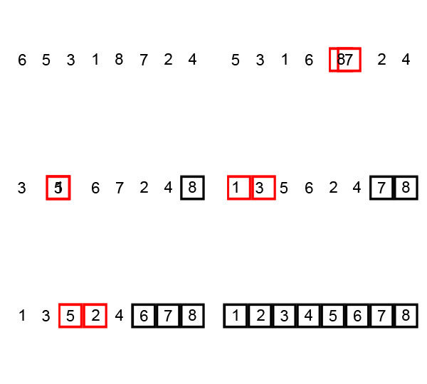
See also: https://www.w3schools.com/dsa/dsa_algo_bubblesort.php

Selection Sort

Given an array $A$ of size $n$, partition the list into “sorted” (initially nothing) and “unsorted” (initially the entire list) parts. Within the unsorted part, find the minimum element and swap it with the first element of the unsorted portion. Then, expand the sorted portion to include this new element. Worst-case runtime: $O(n^2)$; Best-case runtime: $\Omega(n^2)$.

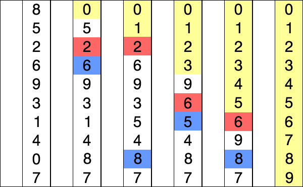
See also: https://www.w3schools.com/dsa/dsa_algo_selectionsort.php

Insertion Sort

Given an array $A$ of size $n$, partition the list into “sorted” (initially nothing) and “unsorted” (initially the entire list) parts. Next, get the first element of the unsorted portion of the list; let $c$ be this value. Then, scan through the sorted portion of the list until you find an index $i$ such that $A[i] \leq c < A[i+1]$, and insert $c$ in between these two values (shifting the values to the right), expanding the sorted portion of the list and shrinking the unsorted portion. Worst-case runtime: $O(n^2)$; Best-case runtime: $\Omega(n)$.

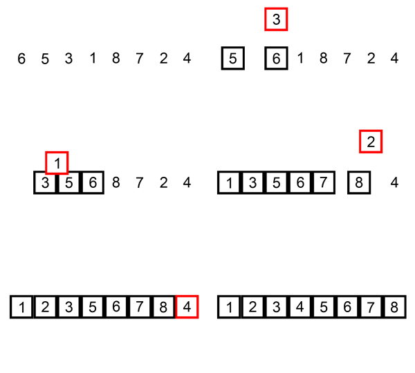
See also: https://www.w3schools.com/dsa/dsa_algo_insertionsort.php

Merge Sort

Given an array $A$ of size $n$, split the array in half. Recursively split each sub-array until arriving at arrays of size $1$. Arrays of size $1$ are trivially sorted. Now, when going down the recursion stack, the left and right sub-arrays are sorted, and you merge these sorted sub-arrays into a new sorted array. Runtime (Best and Worst): $\Theta(n)$.

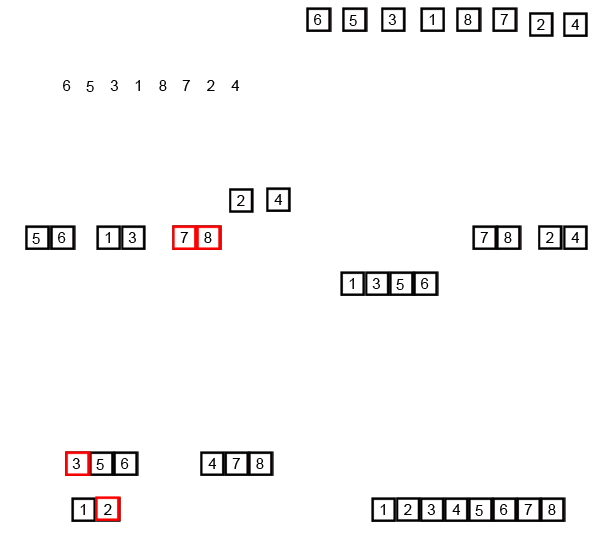
See also: https://www.w3schools.com/dsa/dsa_algo_mergesort.php

Quicksort

Quicksort is actually a family of algorithms which sort a list as follows. Given an array $A$ of size $n$:

• Pick a pivot index $i$ and a pivot value pivot = A[i].
• Partition $A$ into three buckets: all elements of $A$ that are less than pivot, all element of $A$ that are equal to pivot, and all elements of $A$ that are greater than pivot.
• Recursively sort the “less than” and “greater than” buckets.
• Merge the sorted buckets together. In class, we discussed picking $i$ (i.e., pivot) uniformly random from all possible values in the current list. This gives $O(n \log(n))$ time on average, but can have $O(n^2)$ time in the worst case (if you are unlucky). Other pivot selection strategies include (non-exhaustive):
• Always pick the first/middle/last element of the list;
• Pick the median of the first, middle, and last elements.

See also: https://www.w3schools.com/dsa/dsa_algo_quicksort.php

Lecture 1 (Aug. 25, 2026) Sorting Algorithms Review

In this lecture, we briefly reviewed some sorting algorithms (with a more thorough review postponed until Lecture 2). We also reviewed the following important concepts for sorting algorithms.

• Stable vs. Unstable Sort. A stable sorting algorithm preserves the relative order of the list given as input. This is important for sorting data with many attributes. An example is given below.
  • Given a list of tuples of the form ("name", age) as input, sort the list by age. Example list: list = [("Alice", 25), ("Bob", 28), ("Charlie", 25)].
    • Stable sort: outputs the list [("Alice", 25), ("Charlie", 25), ("Bob", 28)]. This is stable because the tuple ("Alice", 25) appeared before ("Charlie", 25) in the original list.
    • Unstable sort: can output either [("Alice", 25), ("Charlie", 25), ("Bob", 28)] or [("Charlie", 25), ("Alice", 25), ("Bob", 28)].
• In-place vs. Not In-place Sort. An in-place sorting algorithm only uses a constant amount of memory to sort the list. Note that this means the sorting algorithm cannot copy the data (as given a list of size $n$, this gives $O(n)$ extra space used). Generally speaking, in-place sorting algorithms are more difficult to implement and often have larger overheads when compared to not in-place sorting, but this can vary.

In-Class Code

In this section, I will post the problems we have tackled in class, as well as the code we wrote to solve the problems. This section will continue to grow throughout the semester. Note that it is posted in reverse chronological order (most recent problems are posted first).

(Sept. 29, 2026) Check Completeness of a Binary Tree

Topic: Trees
Link

# Definition for a binary tree node.
# class TreeNode:
#     def __init__(self, val=0, left=None, right=None):
#         self.val = val
#         self.left = left
#         self.right = right
class Solution:
    # Idea: DFS only down the leftmost path. This is the
    # max possible depth of the tree.
    def max_depth(self, root: TreeNode | None) -> int:
        if(root == None):
            return 0
        return (1+self.max_depth(root.left))
    
    def isCompleteTree(self, root: TreeNode | None) -> bool:
        depth = self.max_depth(root)-1 # Making the root be depth 0

        queue = [root]
        level = 0
        num_nodes = 2**level
        while(len(queue)>0):
            # If we are not at the deepest level of the tree and 
            # we do not have the full amount of nodes, return False
            if(len(queue) != num_nodes and level < depth):
                return False

            # Get all nodes from the current level out of the queue
            curr_level = []
            while(len(queue)>0):
                curr_level.append(queue.pop(0))
            
            # If we are not at the level right above depth, add
            # all children to the queue as in a level-order 
            # traversal or BFS
            if(level < depth-1):
                for node in curr_level:
                    # only add children if they are NOT null/None
                    if(node.left):
                        queue.append(node.left)
                    if(node.right):
                        queue.append(node.right)
            # Now, if we are at depth-1, add EVERY child to the
            # queue, even if they are null/none
            elif(level == depth-1): 
                for node in curr_level:
                    queue.append(node.left)
                    queue.append(node.right)
            else: # level == depth
                # Flag to handle the case that the last level is partially filled.
                # If true, it means that we should only see null/None nodes in the
                # remainder of the queue. Becomes "True" upon seeing the first null/
                # None node.
                noMoreNodes = False
                # Iterate through the current level in-order
                for node in curr_level:
                    if(noMoreNodes):
                        # If we shouldn't see any non-null/-None nodes, and we
                        # see one, return False
                        if(node):
                            return False
                    else:
                        # If the node is None/null, we should ONLY see null/None
                        # nodes in the remainder of the queue
                        if(not node):
                            noMoreNodes = True
                        else:
                            # If any node at level==depth has a child, the tree is
                            # ill-structured and we return false.
                            if(node.left or node.right):
                                return False

            level = level+1
            num_nodes = num_nodes*2

        return True

(Sept. 22, 2026) Construct Binary Tree from Preorder and Inorder Traversal

Topic: Trees.
Link

# Definition for a binary tree node.
# class TreeNode:
#     def __init__(self, val=0, left=None, right=None):
#         self.val = val
#         self.left = left
#         self.right = right
class Solution:
    def buildTree(self, preorder: list[int], inorder: list[int]) -> TreeNode | None:
        if(len(inorder)==0):
            return None
        if(len(inorder)==1):
            return TreeNode(inorder[0])
        rootval = preorder[0]
        root = TreeNode(rootval)
        root_idx = inorder.index(rootval)
        left_inorder_slice = inorder[:root_idx]
        right_inorder_slice = inorder[root_idx+1:]
        left_preorder_slice = preorder[1:1+len(left_inorder_slice)]
        right_preorder_slice = preorder[1+len(left_inorder_slice):]

        root.left = self.buildTree(left_preorder_slice, left_inorder_slice)
        root.right = self.buildTree(right_preorder_slice, right_inorder_slice)

        return root

(Sept. 17, 2026) Binary Tree Traversals II

Topic: Trees.
Level Order Traversal
Level Order Traversal II
Pre-order Traversal

Level Order Traversal: (1) visit myself, (2) visit children in-order from left to right.
Level Order Traversal II: (1) visit all leaf nodes in order from left to right, (2) visit all parents in order from left to right.

# Definition for a binary tree node.
# class TreeNode:
#     def __init__(self, val=0, left=None, right=None):
#         self.val = val
#         self.left = left
#         self.right = right
class Solution:
    def levelOrder(self, root: TreeNode | None) -> list[list[int]]:
        if(root == None):
            return []
        queue = [root]
        res = []
        while(queue):
            lvl = []
            for i in range(len(queue)):
                node = queue.pop(0)
                lvl.append(node.val)
                if(node.left != None):
                    queue.append(node.left)
                if(node.right != None):
                    queue.append(node.right)
            res.append(lvl)

        # Another approach here
        # while len(queue)>0:
        #     lvl = []
        #     for ele in queue:
        #         lvl.append(ele)
        #     for i in range(len(lvl)):
        #         queue.pop(0)
        #     for ele in lvl:
        #         if(ele.left != None):
        #             queue.append(ele.left)
        #         if(ele.right != None):
        #             queue.append(ele.right)
        #     res.append([ node.val for node in lvl ])

        # return reverse(res) -- for Level Order Traversal II
        return res

Pre-order Traversal: in this version of the problem, you were tasked with coming up with a non-recursive algorithm to perform this traversal.

# Definition for a binary tree node.
# class TreeNode:
#     def __init__(self, val=0, left=None, right=None):
#         self.val = val
#         self.left = left
#         self.right = right
class Solution:
    def preorderTraversal(self, root: TreeNode | None) -> list[int]:
        if(root == None):
            return []
        res = []
        stack = [root]
        while(len(stack)>0):
            curr = stack.pop()
            res.append(curr.val)
            if(curr.right):
                stack.append(curr.right)
            if(curr.left):
                stack.append(curr.left)
        return res

(Sept. 15, 2026) Binary Tree Traversals

Topic: Trees.
In-order Traversal
Post-order Traversal

In-order Traversal: (1) visit left subtree, (2) visit self, (3) visit right subtree

# Definition for a binary tree node.
# class TreeNode:
#     def __init__(self, val=0, left=None, right=None):
#         self.val = val
#         self.left = left
#         self.right = right
class Solution:
    def inorderTraversal(self, root: TreeNode | None) -> list[int]:
        if(root==None):
            print("null")
            return []
        L = self.inorderTraversal(root.left)
        print(root.val)
        R = self.inorderTraversal(root.right)
        return L + [root.val] + R

Post-order Traversal: (1) visit left subtree, (2) visit right subtree, (3) visit self

# Definition for a binary tree node.
# class TreeNode:
#     def __init__(self, val=0, left=None, right=None):
#         self.val = val
#         self.left = left
#         self.right = right
class Solution:
    def postorderTraversal(self, root: TreeNode | None) -> list[int]:
        if(root==None):
            print("null")
            return []
        
        L = self.postorderTraversal(root.left)
        R = self.postorderTraversal(root.right)
        print(root.val)
        return L  + R + [root.val]

(Sept. 10, 2026) Majority Element

Topic: Hashing.
Link

Solution with a hashmap

class Solution:
    def majorityElement(self, nums: List[int]) -> int:
        if(len(nums) == 1):
            return nums[0]
        majority = (len(nums)//2)+1
        hashtable = {}
        for num in nums:
            if num in hashtable:
                hashtable[num] += 1
                if(hashtable[num] >= majority):
                    return num
            else:
                hashtable[num] = 1

More clever solution just by smartly counting.

class Solution {
public:
    int majorityElement(vector<int>& nums) {
        int output = 0;
        int majority = 0;
        for(int num: nums) {
            if(majority == 0) {
                output = num;
                majority++;
            }
            else if(num == output) {
                majority++;
            }
            else {
                majority--;
            }
        }
        return output;
    }
};

(Sept. 8, 2026) Two Sum, Longest Substring without Repeating Characters

Topic: Hashing.
Link 1, Link 2

Two Sum

class Solution:
    def twoSum(self, nums: List[int], target: int) -> List[int]:
        # key-value pair (num, index)
        # nums[index] = num
        seen = {} 
        for i in range(len(nums)):
            num = nums[i]
            comp = target-num
            if(comp in seen): # check if comp is a key in seen
                return [i, seen[comp]]
            seen[num] = i
        return []

class Solution {
public:
    vector<int> twoSum(vector<int>& nums, int target) {
        unordered_map<int,int> seen;

        vector<int> indices {-1,-1};

        for(int i = 0; i < nums.size(); ++i) {
            seen[nums[i]] = i;
        }

        for(int i = 0; i < nums.size(); ++i) {
            int comp = target-nums[i];
            if(seen[comp] && seen[comp] != i) {
                indices[0] = i;
                indices[1] = seen[comp];
                break;
            }
        }
        return indices;

    }
};

Longest Substring Without Repeating Characters

Slow solution

class Solution {
public:
    int lengthOfLongestSubstring(string s) {
        // Idea: 2 pointers
        int max_len = 0;

        unordered_set<char> char_set;
        int left = 0;
        for(int right = 0; right < s.size(); ++right) {
            if(char_set.count(s[right]) == 0) {
                char_set.insert(s[right]);
                max_len = max(max_len, (right-left+1));
            }
            else {
                while(char_set.count(s[right])) {
                    char_set.erase(s[left]);
                    ++left;
                }
                char_set.insert(s[right]);
            }
        }

        // Solution using pointers
        // auto left = s.begin();
        // for(auto right = s.begin(); right != s.end(); right++) {
        //     if(char_set.count(*right)==0) {
        //         char_set.insert(*right);
        //         max_len = max(max_len, static_cast<int>(right-left+1));
        //     }
        //     else {
        //         while(char_set.count(*right)) {
        //             char_set.erase(*left);
        //             left++;
        //         }
        //         char_set.insert(*right);
        //     }
        // }

        return max_len;
    }
};

Faster solution

class Solution {
public:
    int lengthOfLongestSubstring(string s) {
        // Idea: 2 pointers
        int max_len = 0;
        int seen_char[256] {};
        int left = 0;
        int diff = 0;

        for(int right = 0; right < s.size(); ++right) {
            ++diff;
            if(!seen_char[s[right]]) {
                ++seen_char[s[right]];
                max_len = (diff > max_len) ? diff : max_len;
            }
            else {
                while(seen_char[s[right]]) {
                    --seen_char[s[left]];
                    ++left;
                    --diff;
                }
                ++seen_char[s[right]];
            }
        }

        return max_len;
    }
};

(Sept. 03, 2026) Wriggle Sort II

Topic: Sorting.
Link

We give both a C++ and a Python solution. In class, the Python solution was faster and used less memory.

class Solution {
public:
    void wiggleSort(vector<int>& nums) {
        sort(nums.begin(), nums.end());
        vector<int> temp(nums.size());
        int end = nums.size()-1;
        for(int i = 1; i < nums.size(); i=i+2) {
            temp[i] = nums[end];
            --end;
        }

        for(int i = 0; i < nums.size(); i=i+2) {
            temp[i] = nums[end];
            --end;
        }
        for(int i = 0; i < nums.size(); ++i) {
            nums[i] = temp[i];
        }
    }
};

class Solution:
    def wiggleSort(self, nums: List[int]) -> None:
        """
        Do not return anything, modify nums in-place instead.
        """
        nums.sort(reverse=True)
        pivot = len(nums) // 2
        smaller_nums = nums[pivot:]
        larger_nums = nums[:pivot]
        nums.clear()
        for i in range(len(larger_nums)):
            nums.append(smaller_nums[i])
            nums.append(larger_nums[i])
        if(len(smaller_nums) > len(larger_nums)):
            nums.append(smaller_nums[-1])

Implementing the above Python code in C++ gives us a solution that beats 100% of all other solutions, while using less memory than ~71% of all other solutions.

class Solution {
public:
    void wiggleSort(vector<int>& nums) {
        int n = nums.size();
        if(n <= 1) return;
        sort(nums.begin(), nums.end(), greater<int>());
        int pivot = nums.size() / 2;
        vector<int> larger(nums.begin(), nums.begin()+pivot);
        vector<int> smaller(nums.begin()+pivot, nums.end());
        nums.clear();
        int i = 0;
        while(i < larger.size()) {
            nums.push_back(smaller[i]);
            nums.push_back(larger[i]);
            ++i;
        }
        if(n%2 == 1) {
            nums.push_back(smaller[i]);
        }
    }
};

(Sept. 01 and 03, 2026) Sort the Jumbled Numbers

Topic: Sorting.
Link

The code for this problem is much easier to implement in Python.

class Solution:
    def sortJumbled(self, mapping: List[int], nums: List[int]) -> List[int]:
        d = 9 # Problem statement tells us that the maximum number of digits is 9
        temp = []
        # Below, we will translate each item num in nums into a tuple 
        # (num, newnum), where newnum is num converted using mapping
        for num in nums:
            if(num == 0): # need to handle the edge case of item == 0
                temp.append((mapping[num], 0))
            else:
                i = 0
                newnum = 0
                while(num // (10**i) > 0):
                    digit = (num // (10**i)) % 10
                    newnum = newnum + mapping[digit]*(10**i)
                    i = i+1
                temp.append((newnum, item))

        # here, we perform radix sort
        buckets = [[] for i in range(10)]
        for i in range(d):
            for tup in temp:
                digit = (tup[0] // (10**i)) % 10
                buckets[digit].append(tup)
            temp.clear()
            for j in range(10):
                size = len(buckets[j])
                for k in range(size):
                    temp.append(buckets[j][k])
                buckets[j].clear()
        return [ tup[1] for tup in temp ]

(Aug. 27, 2026) Two Sum

Topic: Sorting.
Link

/*
Given an unsorted integer array, find a pair with the given sum in it.
• Each input can have multiple solutions. The output should match with 
    either one of them.
• The solution can return pair in any order. If no pair with the given 
    sum exists, the solution should return the pair (-1, -1).
*/

class Solution
{
public:
	pair<int,int> findPair(vector<int> const &nums, int target)
	{
		// Write your code here...
		// Method 1: O(n^2) via checking all possible pairs
		for(int i = 0; i < nums.size(); ++i) {
			for(int j = i+1; j < nums.size(); ++j) {
				int sum = nums[i]+nums[j];
				if(sum == target) {
					return pair(nums[i], nums[j]);
				}
			}
		}
		return pair(-1,-1);
		
		// Method 2: O(n log n) via Sorting
		vector<int> numsCopy(nums);
		std::sort(numsCopy.begin(), numsCopy.end());
		int low = 0;
		int high = numsCopy.size()-1;
		while(low < high) {
			int sum = numsCopy[low]+numsCopy[high];
			if(sum == target) {
				return pair(numsCopy[low], numsCopy[high]);
			}
			else if(sum < target) {
				++low;
			}
			else --high;
		}
		return pair(-1,-1);
	}
};

(Aug. 25, 2026) Sorting Binary Array and Dutch National Flag Problem

Topic: Sorting.
Link 1, Link 2

/*
Given a binary array, in-place sort it in linear time and 
constant space. The output should contain all zeroes, followed by all ones.
*/

class Solution
{
public:
	void sortArray(vector<int> &nums)
	{
        // Method 1: Counting Sort
        // Algorithm:
        //     Count the number of 0s, followed by the number of 1s.
        //     Add the correct number of 0s to the front of the vector,
        //     followed by the correct number of 1s.
        
        int num_0 = 0;
        int num_1 = 1;

        for(int i = 0; i < nums.size(); ++i) {
            if(nums[i] == 0) {
                nums_0++;
            }
            else {
                nums_1++;
            }
        }
        for(int i = 0; i < nums.size(); ++i) {
            if(i < num_0) {
                nums[i] = 0;
            }
            else nums[i] = 1;
        }


        // Method 2: Two Pointers
        // Algorithm:
        //     Have a pointer at the start (left) and end (right) 
        //     of the vector. If start is 1 and end is 0, swap 
        //     and move pointers closer. If left is 1 and right
        //     is 1, decrement right until a 0 is found. Swap for
        //     left = 0 and right = 0.

        int left = 0;
        int right = nums.size();
        while(left < right) {
            if(nums[left] > nums[right]) {
                nums[left] = 0;
                nums[right] = 1;
                ++left;
                --right;
            }
            else if(nums[left] == 0 && nums[right] == 0) {
                ++left;
            }
            else if(nums[left] == 1 && nums[right] == 1) {
                --right;
            }
            else {
                ++left;
                --right;
            }
        }
	}
};

/*
Given an array containing only 0’s, 1’s, and 2’s, 
in-place sort it in linear time and using constant space.
*/

class Solution
{
public:
	void sortArray(vector<int> &nums)
	{
		// Method 1: Counting Sort

        int num_0;
        int num_1;
        int num_2;
        for(int i = 0; i < nums.size(); ++i) {
            switch(nums[i]) {
                case 0:
                    ++num_0;
                    break;
                case 1:
                    ++num_1;
                    break;
                default:
                    ++num_2;
                    break;
            }
        }
        for(int i = 0; i < nums.size(); ++i) {
            if(i < num_0) {
                nums[i] = 0;
            }
            else if(i < num_0 + num_1) {
                nums[i] = 1;
            }
            else nums[i] = 2;
        }


        // Method 2: "Quick" sort
        int pivot = 1;
        int start = 0;
        int end = nums.size()-1;
        int mid = 0;

        while(start <= end) {
            if(nums[mid] < pivot) {
                int tmp = nums[mid];
                nums[mid] = nums[start];
                nums[start] = tmp;
                ++start;
                ++mid;
            }
            else if(nums[mid] > pivot) {
                int tmp = nums[end];
                nums[end] = nums[mid];
                nums[mid] = tmp;
                --end;
            }
            else ++mid;
        }
	}
};

1. A complete binary tree is a binary tree where every non-leaf node has exactly 2 children. If there are $2^n$ leaf nodes, then a complete binary tree has $2^{n+1}-1$ nodes. ↩