Lecture 4

In-class notes: CS 505 Spring 2025 Lecture 4

Recall how we have the notion of a universal Turing machine: a machine that can simulate and solve any problem that any other Turing machine can solve. We’d like to now define a notion that is similar to this where, if you can solve one problem efficiently, then you can use that algorithm to solve a different problem (also efficiently). This leads us to the notion of reducibility.

Reducibility

As above, the idea of reducibility is that if I can solve problem $B$ (i.e., decide the language $B$), then I can use $B$ to solve (i.e., decide) a different language $A$. Moreover, this is efficient: there is only a polynomial overhead in using $B$ to solve $A$.

Definition (Polynomial-time Reducibility). Let $A$ and $B$ be languages. We say that $A$ is polynomial-time reducible to $B$, denoted as $A{\le }_{p}B$ if there exists a function $f$ that is computable in polynomial-time such that $$x\in A⟺f(x)\in B.$$

Lemma 4.1 (Reducibility is Transitive). Let $A$, $B$, and $C$ be languages. If $A{\le }_{p}B$ and $B{\le }_{p}C$, then $A{\le }_{p}C$.

Proof. By definition, there exist functions $f,g$ such that

$$\begin{array}{r}x\in A⟺f(x)\in B\\ y\in B⟺g(y)\in C\end{array}$$

This implies that $x\in A⟺g(f(x))\in C$. Note that both $f$ and $g$ are polynomial-time computable, so the function $g\circ f=g(f(\cdot ))$ is computable in polynomial time. $\square$

Since reducibility is efficient, it immediately tells us that if one of the problems is efficient, then the other is also efficient.

Theorem 4.2. If $A{\le }_{p}B$ and $B\in \mathbf{P}$, then $A\in \mathbf{P}$.

NP-Completeness

NP-Completeness captures the ideas and goals we’ve been building so far: problems in NP that if we can solve, then we can solve any other problem in NP.

Definition ($\mathbf{NP}$-Completeness). Let $L$ be a language. We say thta $L$ is $\mathbf{NP}$-complete if

1. The language is in $\mathbf{NP}$: $L\in \mathbf{NP}$; and
2. The language is $\mathbf{NP}$-hard: $\forall \hat{L}\in \mathbf{NP}$, we have $\hat{L}{\le }_{p}L$.

Notice that there can be languages $L\in \mathbf{EXP}$ such that $L$ is NP-hard, but this would not be NP-complete, unless $L\in \mathbf{NP}$ or $\mathbf{NP}=\mathbf{EXP}$ (which we don’t know is true or not). NP-completeness captures the intuition that if we can use a language to efficiently verify every other language in NP, then this language itself should be efficiently verifiable (otherwise we just verify the other languages directly).

Unhelpful/Useless NP-Complete Language

We’ll now see an example of an NP-complete language which is not helpful for solving problems. This is because, as we’ll see, it is intimately tied to the Turing machine.

Denote by $TMSAT$ the language of all satisfiable Turing machines, defined as $$TMSAT=\{(\alpha ,x,1^n,1^t):\exists w\in \{0,1{\}}^n\text{ s.t. }{M}_{\alpha }(x,w)=1\text{ in at most }t\text{ steps}\}.$$ Here, $1^n$ and $1^t$ denote a string of $n$ (resp., $t$) 1’s. This is a syntactic convention we use to ensure that any machine deciding $TMSAT$ runs in time that is polynomial in $n$ and $t$; whereas if we specified $n$ and $t$ in binary, then the machine would only run in polynomial time with respect to the bit-length of these numbers.

Lemma 4.3. $TMSAT$ is NP-complete.

Proof. Clearly $TMSAT\in \mathbf{NP}$ by definition. The NTM deciding $TMSAT$ takes the input $(\alpha ,x,1^n,1^t)$, guesses the string $w\in \{0,1{\}}^n$ and runs $M_{\alpha }(x,w)$. If $M_{\alpha }$ exceeds $t$ computational steps, output $0$; otherwise, output according to $M_{\alpha }(x,w)$ ($0$ if $0$, $1$ if $1$).

We now show that $TMSAT$ is NP-hard. That is, for any $L\in \mathbf{NP}$, we show $L{\le }_{p}TMSAT$. To do so, we define a function $f$ satisfying: $x\in L⟺f(x)\in TMSAT$. To being, let $p$ and $q$ be polynomials related to the Turing machine which verifies the language $L$. That is, $p$ and $q$ correspond to the Turing machine $M_L$ which on any input $x$ and witness $w\in \{0,1{\}}^{p(|x|)}$ runs in time at most $q(|x|+|w|)$.

Now we define $f(x)$ as follows for any $x\in \{0,1{\}}^{\ast }$.
$$f:x\mapsto (⟨M_L{⟩}_2,x,1^{p(|x|)},1^{q(|x|+p(|x|))}).$$ The tuple $f(x)$ is in $TMSAT$ if there exists $w\in \{0,1{\}}^{p(|x|)}$ such that $M_L(x,w)=1$ in at most $q(|x|+p(|x|))$ steps. Notice that this is trivially true by definition of the NP language $L$. Therefore we have $f(x)\in TMSAT⟺x\in L$. $\square$

This NP-complete language isn’t useful because it’s very definition makes it trivially NP-complete. Moreover, it is inherently tied to the definition of a Turing machine. Intuitively, this says that: if you can compute the Turing machine which verifies the language $L$, then you can compute the Turing machine which verifies the language $L$.

Ideally, we’d like a language that is NP-complete irrespective of the computational model we use. Intuitively, we want to show that the problem itself that is captured by the language is NP-complete, which would tell us that as long as we can solve this problem (and not the Turing machine tied to the problem), then we can solve other problems in NP.

Boolean Satisfiability

The problem we will examine as a candidate for NP-completeness in this light is Boolean Satisfiability. Recall the notion of Boolean variables or Boolean literals $x_1,\dots ,x_n$, which take on True/False values, where we use $1/0$ to denote these values, respectively. Similarly, recall Boolean operations: for example, $\vee$ (logical OR), $\wedge$ (logical AND), $\oplus$ (logical XOR), $\neg$ (logical NOT, denoted as $\overline{x}=\neg x$), etc. Then, a Boolean expression or Boolean formula is an expression involving Boolean variable and operations (e.g., $(\overline{x}\wedge y)\oplus (x\vee z)$). We define the length or size of a Boolean formula to be the number of non-$\neg$ operations in a formula.

For our purposes, we will only consider Boolean formulas which consist of AND, OR, and NOT. It is a well-known fact that these three operations are universal: any Boolean formula can be rewritten as an equivalent formula using only AND, OR, and NOT. Finally, we say that a Boolean formula $\varphi$ is satisfiable if there exists an assignment of the variable $x_1,\dots ,x_n$ such that $\varphi (x_1,\dots ,x_n)=1$.

Now, the language of Boolean Satisfiability is defined as follows. $$SAT=\{⟨\varphi {⟩}_2:\varphi \text{ is satisfiable}\}.$$

How powerful is $SAT$? One measure of its power is the collapse of P vs. NP if we find a polynomial-time algorithm for deciding $SAT$.

Theorem 4.4. $SAT\in \mathbf{P}⟺\mathbf{P}=\mathbf{NP}$.

Cook-Levin Theorem: SAT is NP-complete

In the 1970’s, Cook and Levin independently showed that $SAT$ is NP-complete. This means that if we can find a satisfying assignment for Boolean formulas, we can solve any problem in NP. We’ll begin proving this theorem, then wrap up the proof in the next lecture.

Theorem 4.5 (Cook-Levin). $SAT$ is NP-complete.

Proof. We must show that $SAT\in \mathbf{NP}$ and that $SAT$ is NP-hard. The first task is straightforward. For the second task, at a high level, we must construct a polynomial-time reduction from any language $L$ to an instance of $SAT$. This reduction must have the property that the $SAT$ instance is satisfiable if and only if membership in $L$ is true. Conceptually, we’ll construct a Boolean formula which encodes the correctness of the Turing machine deciding the language $L$. At a high-level, this is a simple task, but the devil is in the details with this reduction.

To begin, we show that $SAT\in \mathbf{NP}$. We give a simple NTM deciding $SAT$. Let $\varphi$ be a Boolean formula and suppose $\varphi$ has $n$ literals $x_1,\dots ,x_n$. Then, the machine $M_{SAT}$ on input $\varphi$ simply guesses a satisfying assignment for $x_1,\dots ,x_n$, checks if $\varphi$ evaluates to $1$ under this assignment, then accepts or rejects accordingly. Clearly, $M_{SAT}$ is a NTM which decides $\varphi$, and the running time of $M_{SAT}$ is clearly polynomial in the length of $\varphi$.

We now turn to showing that $SAT$ is NP-hard. Before doing this, we switch to the convention of single-tape non-deterministic Turing machines. That is, we’ll use the definition of NP languages where $L\in \mathbf{NP}$ if and only if there is a single-tape NTM which decides $L$ in polynomial time. Since, like deterministic machines, many-tape NTMs are (polynomially equivalent to) single-tape NTMs, everything remains in NP.

The idea behind the reduction is the following. Let $L\in \mathbf{NP}$ with single-tape NTM $M_L$ deciding $L$, and consider any $w\in \{0,1{\}}^{\ast }$.¹ The reduction (i.e., the function $f$) will first map the execution of $M_L(u)$ to a table representing this execution. Then, the reduction will specify a Boolean formula that is satisfiabile if and only if this table representing the execution is correct and accepts the input $x$; otherwise the formula will be unsatisfiable.

Assume that on inputs of length $n$, the machine $M_L$ runs in time $n^k$ for some constant $k$ (for convenience in the proof, we actually assume the runtime is $n^k-3$, but this is a minor detail). We’ll construct a table $T$ representing the computation of $M_L(u)$ of size $n^k\times n^k$. Every row of the table has the following properties:

1. The start and end of every row is filled with a special symbol $\#\notin \Gamma$, where $\Gamma$ is the tape alphabet of $M_L$. We’ll index the start of the row by $0$.²
2. For every row $i$, the cells between the start and end $\#$ symbols contain the contents of $M_L$’s single tape, plus its current state $q\in Q$. The current state $q$ is used to represent the current position of $M_L$’s single tape head.
   • If $q$ is at position $j$ in the row for $1\le j\le n^k-1$, then the tape head is reading from position $j+1$ in the table (which corresponds to the tape head being above position $j$ on $M_L$’s tape (here, we start indexing $M_L$’s tape at $1$).
3. The first row of the table (row $0$) always has the starting configuration of $M_L$. This corresponds to the tuple $(\#,q_0,w,\square ,\dots ,\square ,\#)$.

Since $M_L$ runs in time at most $n^k-3$, it can read/write to/from at most $n^k-3$ cells on its work tape. This is exactly the number of slots in a row of table which are dedicated to the work tape configuration, plus 2 slots for $\#$, and one more slot for the current state.

Our goal is to define a Boolean formula $\varphi$ capturing the correctness of the table representing $M_L(w)$. To do this, we first set up the alphabet of the table. Let $C=Q\cup \Gamma \cup \{\#\}$. We call $C$ the table alphabet. We let $cell[i,j]\in C$ denote a cell of the table for all $i,j\in \{0,1,\dots ,n^k-1\}$.

For every cell $cell[i,j]$ and every $s\in C$, we define a unique Boolean literal $x_{i,j,s}$. This literal represents the statement “$cell[i,j]=s$”. In particular, if $cell[i,j]=\square$, then we would set $x_{i,j,\square }=1$, and if $cell[i,j]\ne \square$, then we’d set $x_{i,j,\square }=0$. The reverse is also true; the literal being $1$ means the cell contains that element from $C$, and being $0$ means it does not.

Using these literals, we’ll now encode the correctness of the table for $M_L(w)$ into a Boolean formula $\varphi$. This formula is going to be the conjunction (i.e., logical AND) of 4 sub-formulas: $$\varphi ={\varphi }_{start}\wedge {\varphi }_{accept}\wedge {\varphi }_{cell}\wedge {\varphi }_{move}.$$

The formula ${\varphi }_{start}$ is simple: it will represent the correct starting configuration of the machine. This is a straightforward AND of many literals, shown below: $${\varphi }_{start}=x_{0,0,\#}\wedge x_{0,1,q_0}\wedge x_{0,2,w_1}\wedge \cdots \wedge x_{0,n+1,w_n}\wedge x_{0,n+2,\square }\wedge \cdots \wedge x_{0,n^k-2,\square }\wedge x_{0,n^k-1,\#}.$$

Next, the formula ${\varphi }_{accept}$ will check that the table is an accepting table. That is, it will check that there exists at least one accepting state $q_{accept}$ somwhere in the table. Note that we do not care where this accepting state is, nor if there is also a rejecting state, located in the table; we will handle these consistency checks with ${\varphi }_{move}$. Since all we care about is there is at least one accepting state, we can simply take a large OR of all the cells, yielding: $${\varphi }_{accept}=\underset{1\le i,j\le n^k-2}{\bigvee }{x}_{i,j,q_{accept}}.$$

The formula ${\varphi }_{cell}$ is going to make sure that every cell of the table only contains a single element of $C$. That is, we check to make sure that (1) every cell contains an element of $C$, and (2) every cell only contains a single element of $C$. For (1), we can check this with a simple OR. Let $0\le i,j\le n^k-1$. Then we can check if $cell[i,j]$ contains an element of $s$ using the expression $$\underset{s\in C}{\bigvee }{x}_{i,j,s}.$$ If this is true, we know that $cell[i,j]\in C$.

Now we ensure that $cell[i,j]$ only contains a single value from $C$. This is done by making sure that for all $s,t\in C$ such that $s\ne t$, the expression ${\overline{x}}_{i,j,s}\vee {\overline{x}}_{i,j,t}$ is true. This expression evaluates to false when $cell[i,j]$ contains both $s$ and $t$. If it contains at most one of $s$ or $t$ (including neither of them), then this expression is satisfied. Then we check that this holds over all $s\ne t$. Thus, (2) is captured by the formula= $$\underset{\begin{array}{c}s,t\in C\\ s\ne t\end{array}}{\bigwedge }({\overline{x}}_{i,j,s}\vee {\overline{x}}_{i,j,t}).$$

Therefore, a single cell $cell[i,j]$ is valid if both (1) and (2) hold. We then check that this condition holds for all possible cells, yielding our final expression $${\varphi }_{cell}=\underset{0\le i,j\le n^k-1}{\bigwedge }\left[\left(\underset{s\in C}{\bigvee }{x}_{i,j,s}\right)\wedge \left(\underset{\begin{array}{c}s,t\in C\\ s\ne t\end{array}}{\bigwedge }({\overline{x}}_{i,j,s}\vee {\overline{x}}_{i,j,t})\right)\right].$$

Finally, we turn to the formula ${\varphi }_{move}$. The goal of ${\varphi }_{move}$ is to ensure that the table we’ve constructed is a correct execution of the Turing machine $M_L$ on input $w$. Intuitively, this involves confirming that transitioning from configuration $i$ to $i+1$ was valid (according to the transition function $\delta$ of $M_L$); i.e., that row $i$ in the table is consistent with row $i+1$. Unfortunately, trying to cook up a small (i.e., polynoimal-sized) formula for checking row $i$ vs. $i+1$ of the entire row seems to not be possible (e.g., this could take many logical ORs of some $n^k$-sized sub-formulas). Fortunately, it is enough for us to look at small $2\times 3$ windows of the table representing $M_L(w)$’s computation.

This is (one of the many) beautiful parts of the Cook-Levin theorem. Intuitively, this “looking at windows” to check consistency showcases how highly local Turing machine computations are. As we will see, we will be able to completely verify the entire computation of the Turing machine by scanning over all $2\times 3$ windows in the given table.

For $0\le i\le n^k-1$ and $0\le j\le n^k-3$, define $W_{i,j}$ as the $2\times 3$ the following matrix with entries from $C$: $$W_{i,j}=\left[\begin{array}{ccc}cell[i,j]& cell[i,j+1]& cell[i,j+2]\\ cell[i+1,j]& cell[i+1,j+1]& cell[i+1,j+2]\end{array}\right]$$ We say that window $W_{i,j}$ is legal if this window does not violate the actions of the transition function $\delta$.

Rather than be super formal with this definition (which does not help with intuition), we’ll see some examples of legal windows. First suppose that $a,b,c\in \Gamma$ and let $q_1,q_2$ be states of $M_L$. Now suppose the transition function $\delta$ is defined as follows (for this limited example):

• $\delta (q_1,a)=\{(q_1,b,R)\}$; i.e., while in state $q_1$, if $a$ is read from under the tape head, write $b$ under the tape head, then move the tape head right and stay in state $q_1$.

• $\delta (q_1,b)=\{(q_2,c,L),(q_2,a,R)\}$; i.e., while in state $q_1$, if $b$ is read from under the tape head, non-deterministically choose whether to

  • write $c$ under the tape head, move the tape head left, then change to state $q_2$; or
  • write $a$ under the tape head, move the tape head right, then change to state $q_2$.

With respect to this transition function, the following windows would be considered legal.

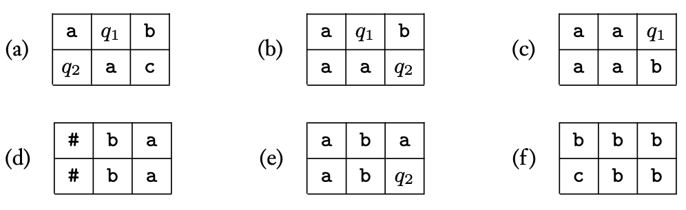
In this figure, windows (a) and (b) are legal because the transition function specifies these are legal actions (recall that the tape head reads the symbol next to the state in the table). Now window (c) is legal because with $q_1$ appearing on the top right, then the symbol $b$ appearing in the bottom right, this was possible if the symbol $a$ were to the right of $q_1$ and then $q_1$ moved right (as specified by $\delta$). Window (d) is legal because the top and bottom are identical, indicating that the tape head is nowhere near these positions and therefore could not have modified them. Also, it is legal for $\#$ to be in the left column (they can also appear in the right column, but never in the center column). Window (e) is legal because state $q_1$ might have been to the immediate right of the top row, a $b$ may have been read, then the tape head may have moved left and transitioned to state $q_2$, which is a valid transition under $\delta$. Finally, window (f) is legal because $q_1$ may be to the immediate left of the first row, read $b$, wrote $c$ then moved left, which is valid under $\delta$.

Now with respect to this transition function, here are examples of illegal windows.

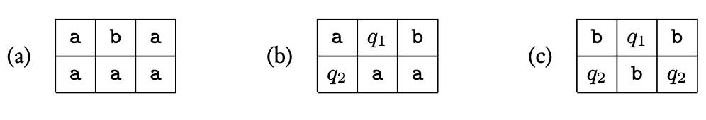
In the above figure, window (a) is illegal since the tape head was not in a position to change $b$ to $a$. Window (b) is illegal since the while in state $q_1$ and reading a $b$, the transition function does not allow the machine to write $a$ then move left and change to state $q_2$. Window (c) is illegal because there are two states specified in the bottom row.

Now, intuitively, we want to specify ${\varphi }_{move}$ as the formula $${\varphi }_{move}=\underset{\begin{array}{c}0\le i<n^k-1\\ 0\le j<n^k-2\end{array}}{\bigwedge }[W_{i,j}\text{ is legal}].$$ This says that all possible windows are legal. In the next lecture, we’ll see that this is enough to show the entire Turing machine computation is valid.