CS 505 - Computability and Complexity Theory
Welcome to the class! I’m excited to have you. Throughout this website, you’ll find all the relevant information needed for the course.
On this page, I’ll post important announcements, as well as a changelog. If you have any questions, please feel free to reach out to me.
Announcements
- [
May 8, 2025] All grades except for the Final Project write-up have been posted to Blackboard. You also should have received feedback in Blackboard for your project presentations (peer feedback and my own feedback). If you have any questions, contact me as soon as possible. Sample solutions for Homework 5 have been posted. Lecture 20 typed notes posted. - [
April 28, 2025] Final Project write-ups are now required to be submitted via Blackboard. This has been noted on the Final Project page, as well as the PDF included there. Typed notes for Lecture 19 posted. - [
April 26, 2025] Handwritten notes for Lecture 23 and Lecture 24 posted. Additional resources for the PCP theorem posted; see Resources. - [
April 21, 2025] Homework 5 posted. Sample solutions for Homework 3 and Homework 4 posted. Make-up office hours will be held this week: April 23, 2025, at 2:00pm (in-person or via Zoom). - [
April 11, 2025] Lecture 21 and Lecture 22 handwritten notes posted. Recorded lectures for Crypto and Complexity Theory, along with handwritten notes for those lectures, posted. Office Hours next week are cancelled due to travel on my end; I will still be available via email or Piazza. - [
April 7, 2025] Lecture 19 and Lecture 20 handwritten notes posted. Schedule updated. Group orderings for the Final Project presentations posted. Please see the webpage for the schedule (i.e., when your group is presenting), along with how the ordering was decided. - [
March 31, 2025] Homework 4 posted. Grades for Homework 3 posted on Gradescope. Schedule updated; no class the week of April 14, instead there will be recorded lectures. - [
March 30, 2025] Typed notes for Lecture 17 and Lecture 18 posted. - [
March 26, 2025] Handwritten notes for Lecture 17 and Lecture 18 posted. Typed notes for Lecture 16 posted. - [
March 17, 2025] Typed notes for Lecture 15 posted. - [
March 16, 2025] Handwritten notes for Lecture 15 and Lecture 16 posted. Typed notes for Lecture 14 posted. Midterm grades posted to Gradescope. - [
March 11, 2025] Final Project information posted. Midterm sample solutions posted to Piazza. Schedule updated with Final Project information. - [
March 3, 2025] Homework 3 posted. Homework 2 sample solutions posted. - [
March 1, 2025] Typed notes for Lecture 13 posted. - [
February 28, 2025] Lecture 11 and Lecture 12 typed notes posted. Handwritten notes for Lecture 13 and Lecture 14 posted. - [
February 23, 2025] Lecture 9 and Lecture 10 typed notes posted. Handwritten notes for Lecture 11 and Lecture 12 posted. - [
February 18, 2025] Schedule updated. - [
February 17, 2025] Lecture 9 and Lecture 10 handwritten notes posted. Homework 1 grades released on Gradescope. Sample solutions for Homework 1 posted. - [
February 13, 2025] Homework 2 posted. - [
February 10, 2025] Lecture 7 and Lecture 8 handwritten notes posted. - [
February 04, 2025] Lecture 5 and Lecture 6 posted. - [
February 03, 2025] Handwritten notes for Lectures 2-6 posted (there are no notes for Lecture 1 since it was written on the board). Lecture 5 and Lecture 6 typed notes will be posted tonight or tomorrow. Zoom link added to office hours (see Important Info below and the Syllabus). - [
January 31, 2025] Homework 1 updated to reflect schedule changes. Problem 5 has been changed. If you do not see this change, you may need to force refresh the course website in your browser, or open it in an incognito window. Schedule updated. - [
January 27, 2025] Lecture 3 and Lecture 4 posted. - [
January 21, 2025] Homework 1 posted. Homework collaboration policy posted. - [
January 20, 2025] In-class lecture on January 21, 2025, is cancelled due to the weather. Class will be held on Zoom. Please check your email for the Zoom link. - [
January 20, 2025] Since today is a holiday and the weather is very cold, in-person office hours are optional. A Zoom link will be sent for office hours today (check your email). - [
January 19, 2025] Lecture 1 and Lecture 2 have been posted. Office hours have been updated (see above or the syllabus).
Important Info
Instructor: Alexander R. Block
Email: arblock [at] uic [dot] edu
Drop-in Office Hours
- Time: Mondays, 2–3pm (or by appointment)
- Location: SEO 1216 or Zoom
- Zoom link (UIC login required): https://uic.zoom.us/j/81305503904?pwd=w4N9MLSrL4M7sny3zQmYyWT6MQgkiG.1
Course Modality and Schedule: In-person only, BSB 289, 2:00 pm - 3:15 pm, Tuesday & Thursday.
Important Links
Changelog
- [
January 20, 2025] Announcements moved to the top of this page. Links to lecture notes added to the schedule and resources. - [
January 19, 2025] Added important info to this page. Announcement on this day posted. - [
January 13, 2025] Syllabus updated. - [
January 06, 2025] Website available.
Syllabus
Instructor and Course Details
Instructor: Alexander R. Block
Email: arblock [at] uic [dot] edu
Drop-in Office Hours
- Time: Mondays, 2–3pm (or by appointment)
- Location: SEO 1216 or Zoom
- Zoom link (UIC login required): https://uic.zoom.us/j/81305503904?pwd=w4N9MLSrL4M7sny3zQmYyWT6MQgkiG.1
Course Modality and Schedule: In-person only, BSB 289, 2:00 pm - 3:15 pm, Tuesday & Thursday.
Blackboard: https://uic.blackboard.com/ultra/courses/_279721_1/cl/outline
Gradescope: https://www.gradescope.com/courses/942742
Piazza: https://piazza.com/uic/spring2025/cs505
Course Announcements
Course information will primarily be conveyed using this website (see here). Course discussion will happen on Piazza. All course assignments and grades will be collected and returned through Gradescope. I will also send email notifications to the class with announcements.
You are responsible for checking this website and emails for any and all updates and information regarding the course, including homework assignments and schedule changes. You are also responsible for keeping up to date on Piazza for any corrections and/or clarifications regarding assignments, or other important information.
Blackboard will be used sparingly in this course, primarily for Homework, Midterm, Final Project, and Final Grades. For all technical questions about Blackboard, email the Learning Technology Solutions team at LTS@uic.edu.
Communication Expectations
Students are responsible for all information instructors send to your UIC email. Faculty messages should be regularly monitored and read in a timely fashion.
Please use Piazza private messages shared with the instructors (not just the professor or TA by name) if you wish to communicate with us directly. Please only use email for something that explicitly should be kept private only to that person.
Please email me if you face an unexpected situation that may impede your attendance, participation in class and exam sessions, or timely completion of assignments.
Course Information
CS 505 is a graduate-level introductory course to Computability and Complexity Theory. You will be expected to read, understand, and write formal (i.e., mathematic) proofs.
Prerequisites: For UIC students, CS 305 is listed as a prerequisite. However, most (if not all) topics covered will be self-contained in this course. As stated above (but in another way), you will need mathematical maturity to succeed in this course. That is, you should be comfortable answering questions of the form “prove or disprove the following statements.” If you are able to do this, then this course is for you; if you struggle with these types of problem, then this course may not be for you.
Brief list of topics to be covered (subject to change)
- Turing machines and their equivalent computational models
- Languages and Decidability
- The class
- The class , and -Completeness
- Randomized Computations
- Space Complexity
- Interactive proofs;
- (Time-dependent) Cryptography and Complexity Theory
Required and Recommended Course Material: No textbook is required for this course. Lectures will have all relevant information.
I will be closely following the book Computational Complexity: A Modern Approach by Aurora and Barak. I will additionally use material from Introduction to the Theory of Computation by Michael Sipser, Mathematics and Computation by Avi Widgerson, and Proofs, Arguments, and Zero-Knowledge by Justin Thaler.
I will give suggested additional readings for each lecture in relevant material freely available online.
Course Copyright: Please protect the copyright integrity of all course materials and content. Please do not upload course materials not created by you onto third-party websites or share content with anyone not enrolled in our course.
The purpose of this syllabus is to give students guidance on what may be covered during the semester. I intend to follow the syllabus as closely as possible; however, I also reserve the right to modify, supplements, and/or make changes to the course as needs arise. All such changes will be communicated in advance through in-class annoucnements and in writing via this website and email.
Course Policies and Classroom Expectations
Grading Policies & Point Breakdown
Grades will be curved based on an aggregate course score and are not defined ahead of time. The score cut-offs for A, B, C, etc., will be set after the end of the course.
The course will have the following grade breakdown:
| Task | % of total grade |
|---|---|
| Homework | 40% |
| Midterm Exam | 25% |
| Final Project | 35% |
Final Grade Assignments
My goal is to ensure that the assessment of your learning in this course is comprehensive, fair, and equitable. Your grade in the class will be based on the number of points you earn out of the total number of points possible, and is not based on your rank relative to other students. There are no set limits to the number of grades given (e.g., everyone can get an A if everyone does well). If the class average is at least 75%, then assigned letter grades will be based on a straight scale with the following thresholds:
| Grade | Threshold |
|---|---|
| A | 90% |
| B | 80–89.9% |
| C | 70–79.9% |
| D | 60–69.9% |
| F | 60% |
If the class mean is less than 75%, then this scale will be adjusted to compensate.
Under no circumstances will grades be adjusted down (except in cases of course policy violation). You can use this straight grading scale as an indicator of your minimum grade in the course at any time during the course. You should keep track of your own points so that at any time during the semester you may calculate your minimum grade based on the total number of points possible at that particular time. If and when, for any reason, you have concerns about your grade in the course, please email me to schedule a time for you to speak with me so that we can discuss study techniques or alternative strategies to help you.
Regrade Policy
You are allowed to request one single regrade per homework assignment/non-final exam. Moreover, with every regrade request, you must submit the following information:
- Which problems you are requesting a regrade for; and
- The exact reason you are requesting a regrade.
I will be strict with this policy to ensure there are no frivolous regrade requests; i.e., do not request a regrade to try and argue for more points. You must have a specific and articulate reason for why you believe something was graded incorrectly. Finally, note that any regrade request can result in a score reduction if additional errors are discovered.
Homework Late Policy
All homework assignments are due by the beginning of class (2:00pm Central Time) on the day they are due. You may submit homework late, with a 25% point reduction per day of being late. On the fourth day of being late, you will receive zero points on the assignment, but it will still be graded in order to give you feedback.
In-class Participation
All course material will be primarily given through in-class lectures. However, as this is a graduate course, I will not require you to attend lecture, but it will be highly encouraged. You are responsible for submitting all assignments, taking the midterm exam, and completing the final project.
Note that though you are not required to attend lecture, I will not answer questions in office hours of the form “can you explain X?” when X was explained in class. By not attending lecture, you do not then get to ask me to teach you the lecture material in office hours.
Evaluation
Homework
There will be 4-5 homework assignments in this course, depending on our progress through the semester. Each homework assignment will be weighted equally when calculating your final grade. See here for more information about completing homework assignments.
Note that your lowest homework score will be automatically dropped from your final grade.
Midterm Exam
There will be an in-class midterm exam, covering topics from (roughly) the first half of the course. The tentative date for the midterm exam is Thursday, March 6, 2025, with an in-class review planned for the previous lecture on Tuesday, March 4, 2025. Please plan to attend class on this day for the midterm exam. I will notify all students once the midterm exam date is finalized, and will do so as soon as possible.
Final Project
In place of a final exam, there will instead be a final project. It will consist of both a written portion and an in-class presentation. Your grade will be assigned based on the written portion, the in-class presentation, and peer-evaluations as well. I will give more details about the final project as we get closer to the midpoint of the semester.
Academic Integrity
Consulting with your classmates on assignments is encouraged, except where noted. However, turn-ins are individual, and copying proofs from your classmates is considered plagiarism. You should never look at someone else’s writing, or show someone else your writing. Either of these actions are considered academic dishonesty (cheating) and will be prosecuted as such.
To avoid suspicion of plagiarism, you must specify your sources together with all turned-in materials. List classmates you discussed your homework with and webpages/resources from which you got inspiration and help. Plagiarism and cheating, as in copying the work of others, paying others to do your work, etc., is obviously prohibited, and will be reported (this includes asking questions and copying answers from forums such as Stack Overflow and Reddit).
I report all suspected academic integrity violations to the dean of students. If it is your first time, the dean of students may provide the option to informally resolve the case – this means the student agrees that my description of what happened is accurate, and the only repercussions on an institutional level are that it is noted that this happened in your internal, UIC files (i.e., the dean of students can see that this happened, but no professors or other people can, and it is not in your transcript). If this is not your first academic integrity violation in any of your classes, a formal hearing is held and the dean of students decides on the institutional consequences. After multiple instances of academic integrity violations, students may be suspended or expelled. For all cases, the student has the option to go through a formal hearing if they believe that they did not actually violate the academic integrity policy. If the dean of students agrees that they did not, then I revert their grade back to the original grade, and the matter is resolved.
If you are found responsible for violating the academic integrity policy, the penalty can range from receiving a zero on the assignment in question, receiving a grade deduction, or receiving an F in the class, depending on the severity of the violation.
As a student and member of the UIC community, you are expected to adhere to the Community Standards of academic integrity, accountability, and respect. Please review the UIC Student Disciplinary Policy for additional information.
GenAI
Since this course will be rigorous in formal (i.e., mathematical proofs), the use of GenAI is NOT allowed. As we will see, there are computational tasks that are impossible in any computational model, thus it is highly likely (and, indeed, expectd) that GenAI would answer any such questions incorrectly.
Failure to adhere to this policy will result in the following consequences:
- First use: You will lose 50% of the points available on the assignment.
- Second use: You will fail the assignment.
- Third use: You will fail the course.
Accommodations
Disability Accommodation Procedures
UIC is committed to full inclusion and participation of people with disabilities in all aspects of university life. If you face or anticipate disability-related barriers while at UIC, please connect with the Disability Resource Center (DRC) at drc.uic.edu, via email at drc@uic.edu, or call (312) 413-2183 to create a plan for reasonable accommodations. To receive accommodations, you will need to disclose the disability to the DRC, complete an interactive registration process with the DRC, and provide me with a Letter of Accommodation (LOA). Upon receipt of an LOA, I will gladly work with you and the DRC to implement approved accommodations.
Religious Accommodations
Following campus policy, if you wish to observe religious holidays, you must notify me by the tenth day of the semester. If the religious holiday is observed on or before the tenth day of the semester, you must notify me at least five days before you will be absent. Please submit this form by email with the subject heading: “[CS 505] YOUR NAME: Requesting Religious Accommodation.”
Classroom Environment
Inclusive Community
UIC values diversity and inclusion. Regardless of age, disability, ethnicity, race, gender, gender identity, sexual orientation, socioeconomic status, geographic background, religion, political ideology, language, or culture, we expect all members of this class to contribute to a respectful, welcoming, and inclusive environment for every other member of our class. If aspects of this course result in barriers to your inclusion, engagement, accurate assessment, or achievement, please notify me as soon as possible.
Name and Pronoun Use
If your name does not match the name on my class roster, please let me know as soon as possible. My pronouns are [she/her; he/him; they/them]. I welcome your pronouns if you would like to share them with me. For more information about pronouns, see this page: https://www.mypronouns.org/what-and-why.
Community Agreement/Classroom Conduct Policy
- Be present by removing yourself from distractions, whether they be phone notifications, entire devices, conversations, or anything else.
- Be respectful of the learning space and community. For example, no side conversations or unnecessary disruptions.
- Use preferred names and gender pronouns.
- Assume goodwill in all interactions, even in disagreement.
- Facilitate dialogue and value the free and safe exchange of ideas.
- Try not to make assumptions, have an open mind, seek to understand, and not judge.
- Approach discussion, challenges, and different perspectives as an opportunity to “think out loud,” learn something new, and understand the concepts or experiences that guide other people’s thinking.
- Debate the concepts, not the person.
- Be gracious and open to change when your ideas, arguments, or positions do not work or are proven wrong.
- Be willing to work together and share helpful study strategies.
- Be mindful of one another’s privacy, and do not invite outsiders into our classroom.
Furthermore, our class (in person and online) will follow the CS Code of Conduct. If you are not adhering to our course norms, a case of behavior misconduct will be submitted to the Dean of Students and to the Director of Undergraduate Studies in the department of Computer Science. If you are not adhering to our course norms, you will not get full credit for your work in this class. For extreme cases of violating the course norms, credit for the course will not be given.
Student Parents
I know well how exhausting balancing school, childcare, and work can be. I would like to help support you and accommodate your family’s needs, so please don’t keep me in the dark. I hope you will feel safe disclosing your student-parent status to me so that I can help you anticipate and solve problems in a way that makes you feel supported. Unforeseen disruptions in childcare often put parents in the position of having to choose between missing classes to stay home with a child or leaving them with a less desirable backup arrangement. While this is not meant to be a long-term childcare solution, occasionally bringing a child to class in order to cover gaps in care is perfectly acceptable. If your baby or young child comes to class with you, please plan to sit close to the door so that you can step outside without disrupting learning for other students if your child needs special attention. Non-parents in the class, please reserve seats near the door for your parenting classmates or others who may need to step out briefly.
Academic Success, Wellness, and Safety
We all need the help and the support of our UIC community. Please visit my drop-in hours for course consultation and other academic or research topics. For additional assistance, please contact your assigned college advisor and visit the support services available to all UIC students.
Academic Success
- UIC Tutoring Resources
- College of Engineering tutoring program
- Equity and Inclusion in Engineering Program
- UIC Library and UIC Library Research Guides.
- Offices supporting the UIC Undergraduate Experience and Academic Programs.
- Student Guide for Information Technology
- First-at-LAS Academic Success Program, focusing on LAS first-generation students.
Wellness
-
Counseling Services : You may seek free and confidential services from the Counseling Center at https://counseling.uic.edu/.
-
Access U&I Care Program for assistance with personal hardships.
-
Campus Advocacy Network : Under Title IX, you have the right to an education that is free from any form of gender-based violence or discrimination. To make a report, email TitleIX@uic.edu. For more information or confidential victim services and advocacy, visit UIC’s Campus Advocacy Network at http://can.uic.edu/.
Safety
- UIC Safe App—PLEASE DOWNLOAD FOR YOUR SAFETY!
- UIC Safety Tips and Resources
- Night Ride
- Emergency Communications: By dialing 5-5555 from a campus phone, you can summon the Police or Fire for any on-campus emergency. You may also set up the complete number, (312) 355-5555, on speed dial on your cell phone.
Schedule
This schedule is tentative and subject to change. Any changes will be announced.
| Lecture Number (Date) | Topics | Announcements | Additional Resources |
|---|---|---|---|
| Lecture 1 (Jan 14) |
| ||
| Lecture 2 (Jan 16) |
| Correction from in-class lecture; see Lecture 2. | |
| Lecture 3 (Jan 21) |
| Homework 1 assigned. | |
| Lecture 4 (Jan 23) |
| ||
| Lecture 5 (Jan 28) |
| ||
| Lecture 6 (Jan 30) |
| Problem 5 of Homework 1 will be changed to reflect change in schedule. | |
| Lecture 7 (Feb 4) |
| ||
| Lecture 8 (Feb 6) |
| Homework 1 due. | |
| Lecture 9 (Feb 11) |
| ||
| Lecture 10 (Feb 13) |
| Homework 2 assigned. | |
| Lecture 11 (Feb 18) |
| ||
| Lecture 12 (Feb 20) |
| ||
| Lecture 13 (Feb 25) |
| ||
| Lecture 14 (Feb 27) |
| Homework 2 due. | |
| Midterm Review (Mar 4) | Covers Lectures 1-13 (Up to and Alternation) | Homework 3 assigned. | |
| Midterm Exam (Mar 6) | Covers Lectures 1-13 | ||
| Lecture 15 (Mar 11) |
| Final Project information posted. | |
| Lecture 16 (Mar 13) |
| ||
| Lecture 17 (Mar 18) |
| ||
| Lecture 18 (Mar 20) |
| Homework 3 due. | |
| Mar 22, 11:59pm CDT | Final Project proposals due. | ||
| NO CLASS; SPRING BREAK (Mar 25) | |||
| NO CLASS; SPRING BREAK (Mar 27) | |||
| Lecture 19 (Apr 1) |
| Homework 4 assigned. | |
| Lecture 20 (Apr 3) |
| ||
| Lecture 21 (Apr 8) |
| ||
| Lecture 22 (Apr 10) |
| ||
| NO CLASS; Recorded Lecture (Apr 15) |
| Homework 4 due. | |
| NO CLASS; Recorded Lecture (Apr 17) |
| ||
| Lecture 23 (Apr 22) |
| Homework 5 assigned. | |
| Lecture 24 (Apr 24) |
| ||
| Final Project Presentations (Apr 29) | |||
| Final Project Presentations (May 1) | |||
| May 6, 2:00pm CDT | Homework 5 due. | ||
| May 10, 11:59pm CDT | Final Project written reports due. |
Resources
This page will be updated throughout the semester with new resources as I find them. If you have found a particularly useful resource, feel free to let me know and I will gladly add them to the resources below.
Lecture Notes
- Lecture 1
- Lecture 2
- Lecture 3
- Lecture 4
- Lecture 5
- Lecture 6
- Lecture 7
- Lecture 8
- Lecture 9
- Lecture 10
- Lecture 11
- Lecture 12
- Lecture 13
- Lecture 14
- Lecture 15
- Lecture 16
- Lecture 17
- Lecture 18
- Lecture 19
- Lecture 20
- Lecture 21
- Lecture 22
- Lecture 23
- Lecture 24
- Crypto and Complexity Theory
Books
- Computational Complexity: A Modern Approach (Draft) by Sanjeev Arora and Boaz Barak
- Introduction to the Theory of Computation1 by Michael Sipser
- Proofs, Arguments, and Zero-knowledge by Justin Thaler
- Mathematics and Computation by Avi Widgerson
Other Lecture Notes and Videos
- Michael Sipser’s Theory of Computation Course at MIT
PCP Theorem
- Notes from Jon Katz: first lecture and second lecture. All his other notes from this course: website.
- Dana Moshkovitz’s Tale of the PCP Theorem.
- Irit Dinur’s alternative proof of the PCP Theorem: The PCP Theorem by Gap Amplification.
- PCP Theorem Course by Irit Dinur and Dana Moshkovitz: Probabilistically Checkable Proofs.
-
You may be able to find the book online for free. I cannot confirm or deny the availability. Supplemental readings may be given from this book and will be paired with the appropriate video lecture from Michael Sipser’s course below. ↩
Homework
This page will be updated with homework assignments as they become available throughout the semester. All homework assignments will be due before the start of class. That is, by no later than 2:00pm Central US Time.
All homework is required to be typeset in .
Included with each assignment is a .pdf file of the assignment, along with a .zip folder with the source for you to use to complete the assignment.
All homework is required to be submitted through Gradescope.
For submission, you will simply need to upload the .pdf file of your assignment.
You will likely not be able to answer all the questions in a given homework when it is released. My intention is to spread out the material you need to complete each homework over several lectures. This will allow you to either (a) do the homework problems incrementally as we cover the relevant material in class; (b) wait until all lectures are completed then do the homework all at once; or (c) finish the homework as soon as it’s assigned by reading ahead in other resources.
The schedule below is tenative and is subject to change based on how we progress through the semester.
Collaboration between sutends is encouraged. However, all collaborations need to be acknowledged (whether they are in this class, or outside of this class). You MUST list all collaborators for homework assignments. Moreover, collaborating does not mean you can copy-paste work from each other. Each submission needs to be in your own words, otherwise it will be considered plagiarism.
You are allowed to look to other resources for help with the homework, but you MUST properly cite these sources.
Please use the \cite command and add your citations in the proper format to the included local.bib in your homework assignments.
Finally, please acknowledge any other discussions that helped you complete this assignment. This can include “office hours,” “Piazza,” or other discussions where direct collaboration did not happen.
Failing to adhere to the collaboration policy outlined above will result in various penalties.
First violation: You will lose 50% of the points available on the assignment.
Two or more violations: You will fail the assignment.
Homework 1
Date Assigned: January 21, 2025.
Due Date: February 6, 2025, no later than 2:00pm Central Time.
Updated: January 31, 2025 (see Announcements).
PDF file: homework-1.pdf (SHA256: bfcb1bb09bcb433c2e22b462bd1a9ea62d227767936db3099261afcfa3124a37)
Source files: homework-1.zip (SHA256: 73fedc2f3141d71314fe451f2732bf6a7c1dcbf14df8d14c0de05d24289d69d4)
Sample solutions: homework-1-solutions.pdf
Homework 2
Date Assigned: February 13, 2025.
Due Date: February 27, 2025, no later than 2:00pm Central Time.
PDF file: homework-2.pdf (SHA256: 38ade5b4a4b5abd0070c33953861e201253efbcd5fc32dc904abc1314a4a1e54)
Source files: homework-2.zip (SHA256: 5e55f481dcc61aa5489875fc1e00084b1b02081c98fb6657d74551c543276b8b)
Sample solutions: homework-2-solutions.pdf
Homework 3
Date Assigned: March 4, 2025.
Due Date: March 20, 2025, no later than 2:00pm Central Time.
PDF file: homework-3.pdf (SHA256: 276a2dea7f34c264b355968bc90c7052889816082c7c1c179566c9b25537d980)
Source files: homework-3.zip (SHA256: 6e9e6b22715ba055dd1a884bdc18078851629992db7a628051c5ccc41d263635)
Sample solutions: homework-3-solutions.pdf
Homework 4
Date Assigned: April 1, 2025
Due Date: April 15, 2025, no later than 2:00pm Central Time.
PDF file: homework-4.pdf (SHA256: c1d1204ea77d579a379c6d25efb81fffcfc769317e754046a9b2e49ab69a1f31)
Source files: homework-4.zip (SHA256: 75ad92909df75544821d88a3a529bf07d6c7748c31b0114c9ba2df1104bcf7ed)
Sample solutions: homework-4-solutions.pdf
Homework 5
Date Assigned: April 22, 2025
Due Date: May 6, 2025, no later than 2:00pm Central Time.
PDF file: homework-5.pdf (SHA256: 01a81895717cab5d20fe83c7506f7293a02586af0fa53084c2865c5c6d1cf40c)
Source files: homework-5.zip (SHA 256: 19aeb9c23d39e0827c41b72213d6f64851bfa3ee5644e3477a50800565e00b9e)
Sample solutions: homework-5-solutions.pdf
Final Project
Final Project Group Presentation Schedule
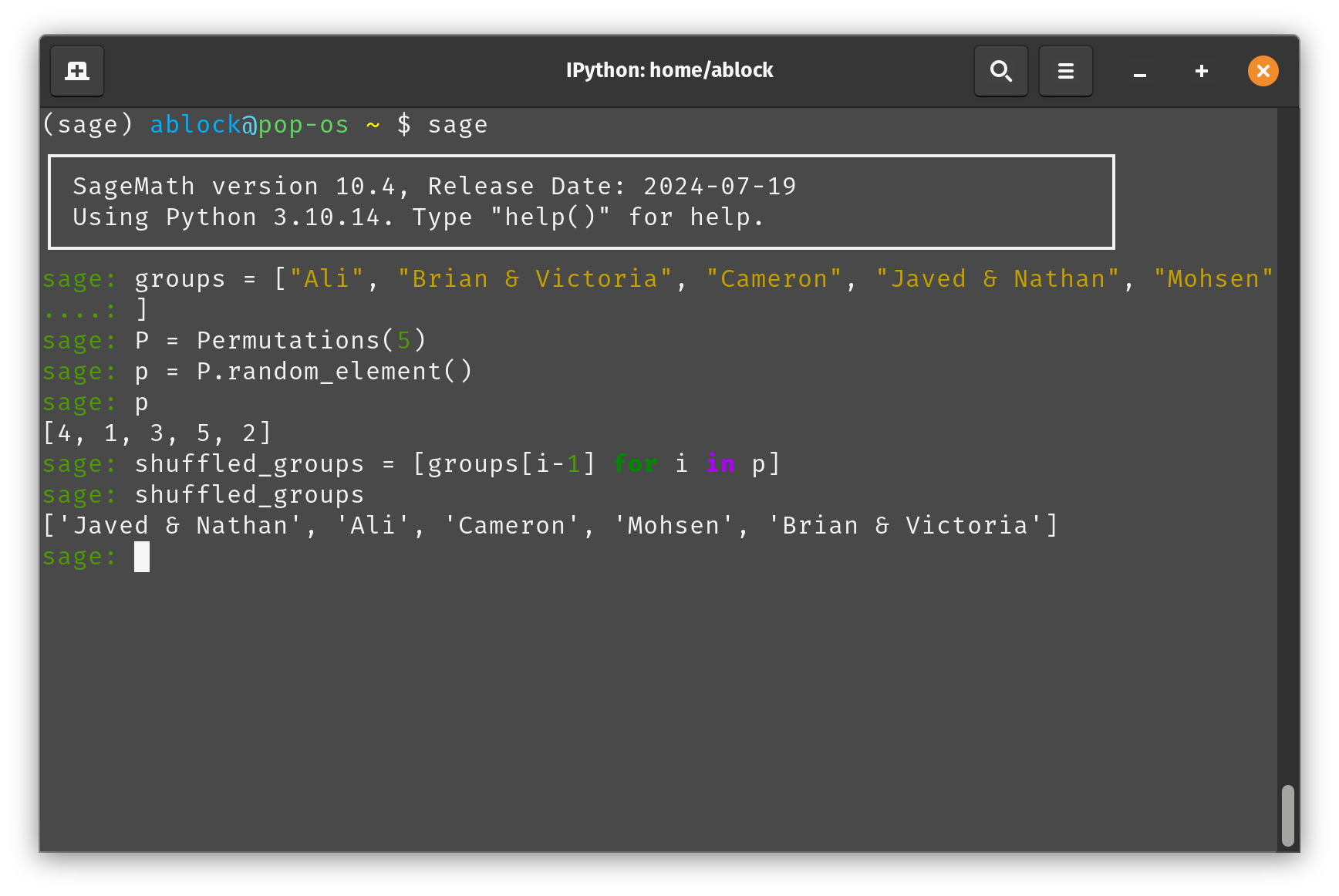
I have randomly generated the Final Project Presentation schedule, as outlined below. The methodology is as follows.
- List all groups in alphabetical order by first name, with each group being sorted alphabetically by first name internally.
- Randomly generate a permutation to shuffle this alphabetical ordering.
- Output the shuffled ordering. First 3 groups present on Tuesday, April 29, 2025; last 2 groups present on Thursday, May 1, 2025.
Groups
- Ali
- Brian & Victoria
- Cameron
- Javed & Nathan
- Mohsen
Random permutation sampled: [4, 1, 3, 5, 2].
Final Ordering
Tuesday, April 29, 2025
- Javed & Nathan
- Ali
- Cameron
Thursday, May 1, 2025
- Mohsen
- Brian & Victoria
Sagemath Code used to generate this result.
groups = ["Ali", "Brian & Victoria", "Cameron", "Javed & Nathan", "Mohsen"]
P = Permutations(5) # set of all permutations on [1,2,3,4,5]
p = P.random_element() # samples a random permutation of the list [1,2,3,4,5]
p # prints the sampled permutatation
shuffled_groups = [groups[i-1] for i in p]
shuffled_groups # prints the new ordering for 'groups'
Code screenshot below.
Project Description
The project you choose can be related to your research area, or completely unrelated. You may work in teams of up to 3 people. However, whatever your project is and however many people you have on your team, the project will consist of two major components—an In-Class Presentation, and a Written Report—as well as two minor components—Project Proposals and Peer Evaluations. There are no rigid page limits for the report; anything between 4–20 pages can work. For the In-Class presentation, you are expected to give a 15–18 minute presentation using the presentation materials of your choice (e.g., PowerPoint, Keynote, , Google Slides, a Board Talk, etc.).
The project can be a survey of a problem or topic of your choice, or a novel analysis of a problem that you like. In the first case, if you read some papers and summarize them in a survey, give the reader the required background (which may be covered only briefly in some conference papers) together with the main results and their proofs and open questions. For the second scenario, if you try to solve a problem that you are interested in, explain the connections with previous work; in case you don’t arrive to a solution by the end of the term, show what approaches you tried and what didn’t work.
The goal of the project is to understand a problem as much as possible, and to give you experience with complexity theory research. Give the reader the background and necessary explanations to make the problem very clear, understand the contribution of the paper, and the approaches used. You do not have to summarize every theorem in the paper (in either write-up or presentation). Pick instead one or a couple of results in the paper(s) you are reading and focus on those, while trying to answer questions such as: What is the idea of the proof? What techniques are the authors using? Where are the difficulties? What are the remaining open questions?
Recent proceedings of good conferences that publish theoretical work are a possible starting point. Some examples are STOC/FOCS/ITCS/SODA/APPROX-RANDOM, CRYPTO/TCC, EC (Economics and Computation), COLT, PODC.
Project Timeline
-
Saturday, March 22, 2025, by 11:59pm CDT. Submit your project proposals to me. This includes at least one paragraph about your project, along with at least one (or, ideally, a few) papers you plan to read for the project. The easiest way to do this is to email me, cc your team members, and include the relevant information in the email.
-
Tuesday, April 29, 2025, and Thursday, May 1, 2025. The last week/last two classes, we will hold the in-class presentations. Attendance will be required except for special cases. Part of this project is to give you experience presenting material you may not be very familiar with or an expert in to an audience who will be even less familiar with your topic. Also, you will be giving peer evaluations to your fellow students as well, and everyone will be required to submit these peer evaluations.
-
Saturday, May 10, 2025, by 11:59pm CDT. Your written reports are due the day after finals. I want to give you as much time as possible for the written reports, but I will still need to read and grade them before grades are due. Early submissions (e.g., before finals) are also fine. You will submit your written reports via
GradescopeBlackboard.
Grade Brakedown
- (5%) Project Proposals
- (10%) Peer Evaluations
- (40%) In-Class Presentation
- (45%) Written Report
Lecture 1
Review
Math Notation
Here are some common math notations we will be using throughout the semester. Any other notation introduced in lecture outside what is presented here will be explained. Please do not be afraid to ask questions about notation in class.
We let denote the set of all integers and let denote the set of natural numbers (i.e., non-negative integers). The set denotes the set of all positive integers. We let denote the set of all real numbers, with and defined to be the ceiling and floor of , respectively (i.e., round up or round down to the nearest integer). All logarithms are base 2 unless otherwise stated; i.e., . When need, we let denote the natural logarithm.
Sets and Strings
Let be a finite set. We say that is a string with alphabet if it is a finite ordered tuple with elements in . That is, if has length , then (i.e., it is a vector). We let denote the set of all finite length strings with alphabet (i.e., the set of all finite length vectors with elements in ). Given two strings and , we let denote their concatenation; sometimes, we also use or to denote their concatenation as well. Finally, given a string/vector , we let denote the length of the string (i.e., number of elements in ). When needed, we let denote the bit-length of ; that is, the number of bits needed to represent . If , then .
Languages
Much of this course will be concerned with the idea of a language. A language is simply a set . A language can be finite or infinite. While the above definition doesn’t really mean much, we’ll see later in the course how we define languages in more meaningful ways.
Function Notation
Let and be arbitrary sets (not necessarily finite). Then we let denote a function from to .
Big-Oh Notation
Let be two functions. We way that is big-oh of if there exists and constant such that for all , we have . We denote this as or . Similarly, we say that is big-omega of if ; we denote this as . We say that is theta of if and .
We say that is little-oh of if for all constants , there exists such that for all , it holds that . We denote this as . Similarly, is litte-omeaga of if ; equivalently, for all constants , there exists such that for all , it holds that . We denote this as .
Turning Machines
The goal of complexity theory is to quantify and measure computational efficiency. How can we do this? It is first necessary to establish a concrete model of computation. But this seems impossible—surely, there are infinite computational models one can cook up to get the job done, right?
Fortunately, we can focus on a single model of computation: the Turning Machine. For (nearly)1 every physically realizable system we have been able to come up with, the Turing machine can efficiently simulate this other model. This gives us a single model with which we can try to understand and quantify computational efficiency.
Turing Machines, Informally
Turing machines, introduced by Alan Turing in 1948, are an attepmt to formalize the idea of computation as people have understood it for centuries. Intuitively, when someone asks you to compute the answer to a problem, we as people seem to follow a basic formula for realizing this:
- Get the problem, along with the inputs to the problem.
- Get a piece of scratch paper to work on.
- Apply a set of rules to the inputs and make decisions according to those rules.
- Arrive at an answer to the problem, state the answer, and stop working.
As a concrete example, consider the problem of multiplying two integers. Take and and suppose we want to compute their product . There is a simple (so-called “grade-school”) algorithm for computing , which we show in the figure below.

Turing machines attempt to formalize the above intuitive process, but in a very restricted capacity (i.e., Turing machines are incredibly simple and, in a word, stupid).
Turing Machines, Formally
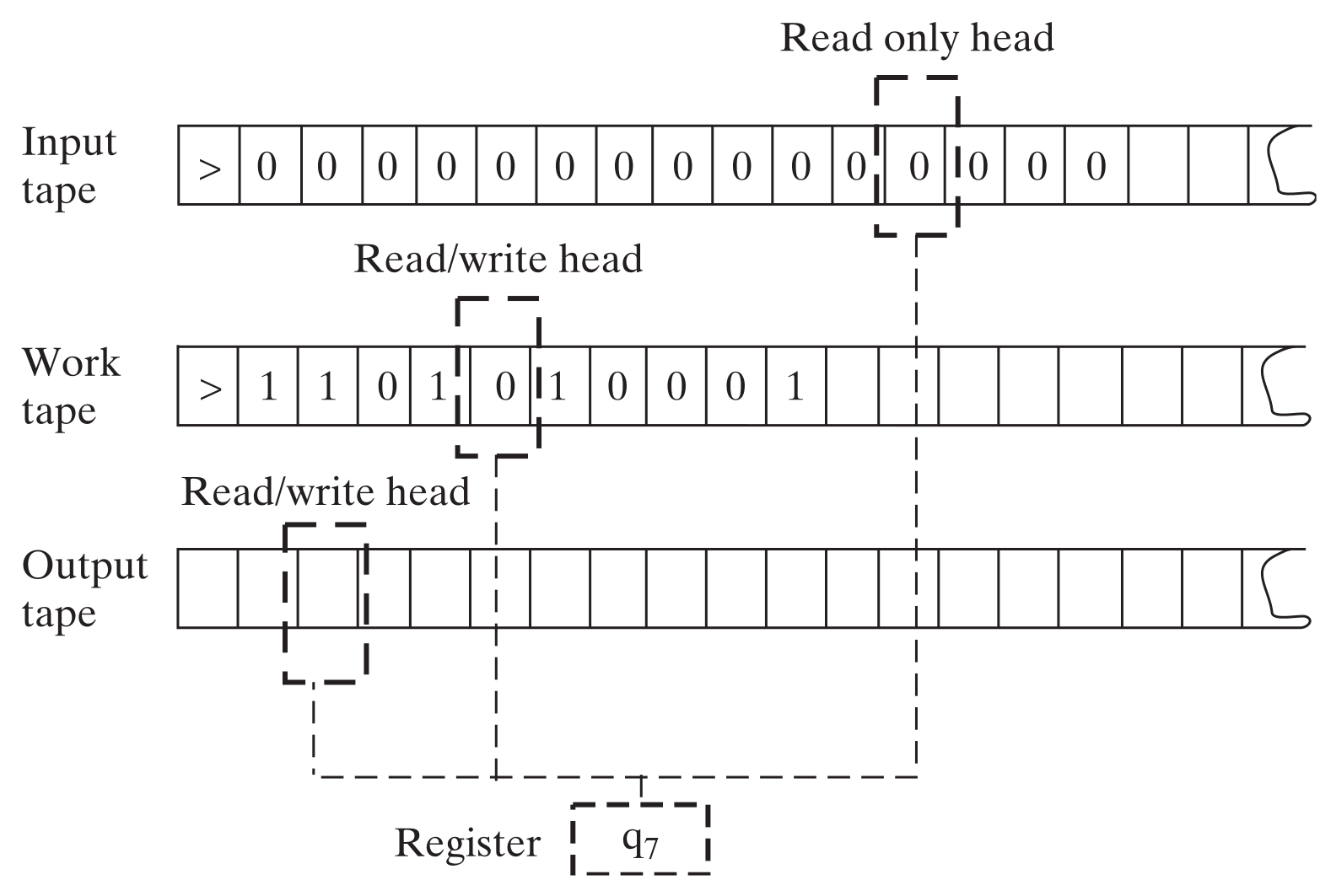
A -tape Turing machine, which we denote by , is a machine with tapes that are infinitely long in one direction (i.e., they are represented by the set ). The machine has a single read-only input tape, a single read-write output tape, and read-write work tapes. also contains a register which tracks the machine’s state. Each head can be moved independently. More formally, a -tape Turing machine is described by a tuple with the following properties:
- is a finite set, which we call the input alphabet;
- is called the tape alphabet, and it contains along with two special symbols that are not in . is the start symbol and is the blank symbol.
- is a finite set of states which can be held in the register. always contains two special states: (the start state) and (the halt state).
- A transition function describing the rules follows during a computation.
We say that a tuple is a configuration of the Turing machine . In this light, the transition function maps configurations of the Turing machine to new configurations as follows:
- represents the current state of the machine stored in its register;
- represents the current symbol under tape ’s head, for ;
- reads the current state and the contents of the tape heads.
It then outputs a new configuration , where
- is the new state stored in the register;
- is a new symbol that is written under the th tape head for (i.e., it excludes the input tape); and
- specifies moving tape head one space Left, one space Right, or telling the tape head to Stay.2
- If the Turing machine is ever in the state , it stops executing the transition function and halts.
Additionally, all Turing machines satisfy the following.
- All tapes are initially set with in every location.
- The first index of every tape is then initialized to . All tape heads begin here.
- On input , all Turing machines will:
- Move the input head , then write to the input tape.
- Move the input head until it reaches .
- Set the initial state in the register to . The Turing machine is now ready to begin its computation.
We call this the initial configuration of the Turing machine.
A graphical example of a -tape Turing machine is presented below.
Turing machine example: Palindromes
Let’s see an example of a Turing machine in action. We will be using Turing machines to compute functions. Let be a function such that if and only if is a palindrome. That is, ; equivalently, if , then for all . Let’s design a Turing machine for computing .
High-level TM Specification. Let be a -tape Turing machine (1 input, 1 output, 1 work tape). On input for any , will do the following.
-
Copy the input to the work tape.
-
Move the input head to the start of the input tape (with under the head), leave the work head at the last position (with under the head).
-
Move the input head one position right (with under the head) and move the work head one position left (with under the head).
-
Read the symbols under the input head and the work head.
(a) If the symbol under the input head is and the symbol under the work head is , then write to the output tape and halt.
(b) Else if the symbols under the input head and work head are not equal, write to the output tape and halt.
(c) Else (i.e., the symbols are equal) move the input head one step right and move the work head one step left.
Formal TM Specification of above. We now formalize thie above process. To do so, we specify (1) the input alphabet; (2) the set of states for ; and (3) the transition function for .
- The input alphabet is simply . This tells us our tape alphabet is .
- The set of states will be .
- The transition function is defined as follows.
Let be a configuration given as input to .
- If , move both the input head and work head right and change the state to .
- If , then read the symbol under the input head (i.e., read ).
- If , write to the current position of the work tape. Then move both the input head and work head one step right. Keep the state as . In this case, the output of the transition function is .
- If , then move the input head left and change the state to . In this case, the output of the transition function is .
- If , read the symbol under the input head (i.e., ).
- If , then move the input head left and keep the state as . In this case, the output of the transition function is .
- If , then move the input head right, move the work head left, and change the state to . In this case, the output of the transition function is .
- If , read what’s under the input and work heads (i.e., and ).
- If and , then write on the output tape and change the state to . In this case, the transition function outputs .
- Else if , then write on the output tape and change the state to . In this case, the transition function outputs .
- Else (i.e., ), then move the input head right and the work head left, keeping the state as . In this case, the transition function outputs .
Turing Machine Equivalences
At first, the Turing machine model seems like a very restrictive model that cannot compute many things, especially real-life computers. However, as we will see, this restrictive computational model is (roughly) equivalent to nearly every other computational model people have thought of over the years. This includes:
- Random access machines;
- Turing machines with write-only output tapes;
- -calculus;
- Single-tape Turing machines;
- Turing machines with bidirectional infinite tapes;
- Pointer and Counter machines;
- Turing machines with only binary input alphabets;
- Oblivious Turing machines.
In the next lecture or two, we will quantify what we mean by Turing machines being equivalent to the above notions.
-
Quantum computers are the one (almost) physically realizable computational model that we have which does not seem to admit efficient simulation on Turing machines. ↩
-
If the Turing machine specifies that a tape head to move left, but it’s at the start of the tape, the head simply stays in the same place. ↩
Lecture 2
In-class notes: CS 505 Spring 2025 Lecture 2
Measuring Runtime of Turing Machines
With the definition of Turing machines established, we can turn towards quantifying the run-time of Turing machines. Informally, the run-time of a Turing machine computing some function is the maximum amount of time needed to compute on all inputs (of a fixed length), where our measure of time corresponds to how many executions of the transition function needs to utilize to compute . First, we need to actually define what it means for a Turing machine to compute a function .
Definition (Turing Machine Computation). Let be a function and let be a Turing machine. We say that computes if for all , when is initialized with input it halts with on the output take. We denote this as .
Now we can define the run-time of a Turing machine computing a function .
Definition (Turing Machine Run-time). Let be a function and let be a Turing machine which computes . Furthermore, let be a function. We say that computes in time if in at most steps for all (i.e., steps). Here, a step of the Turing machine is a single execution of its transition function .
In essence, executing one step of the transition function of a Turing machine is the atomic Turing machine operation.
Time Constructible Functions
An important concept is the idea of time constructible functions, which we will use to quantify and show equivalences among different Turing machine models. It will also be used in later topics (e.g., time hierarchy theorems).
Definition (Time Constructible Function). Let be a function. Then we say that is time construictible if and only if (1) ; and (2) there exists a Turing machine such that for all , we have in time . Here, denotes the binary representation of .
Examples of time constructible functions include Notably, , or any , are not time constructible.
The above examples of non-time constructible functions highlight a key idea behind time constructibility: a Turing machine (usually) needs to read its entire input in order to compute a function. The stipulation allows for a Turing machine to at least read the entire input before computing . If this restriction is removed, then is still time constructible (you simply ignore all inputs and write the constant to the output tape), but remain non-time constructible since the Turing machine is expected to compute in less time than it takes to read !
Turing Machine Equivalences
A function being time constructible turns out to be a key factor in how we define equivalences among Turing machines (and other models as well).1 Informally, we say that a computational model is equivalent to a computational model if any for any computation capable of being performed in can be performed in (with at most polynomial time overhead). In the context of Turing machines, we say that a computational model is equivalent to the Turing machine model if any problem solvable in time in model can be solved by a Turing machine running in time for constant . Intuitively, if is a program in computational model running in time , then a Turing machine will simulate model in order to run program (e.g., similar to modern interpreted programming languages like Python). If runs in time , and is not time constructible, then this simulation will not meet our requirements; i.e., it will not be an efficient simulation.
As mentioned in Lecture 1, the -tape Turing machine model we have been working with is equivalent to many other Turing machine (and non-Turing machine) models. We state these relations formally below.
First, recall that it is sufficient to consider a Turing machine which only uses a binary alphabet.
Lemma 2.1. For every and time constructible , if is computable in time by a Turing machine with tape alphabet , then it is computable in time by a Turing machine with tape alphabet .
Proof Sketch. The main idea is to encode the (non-start and non-blank) symbols of using bits. This requires roughly bits to uniquely encode in binary. Then the new Turing machine simply encodes each symbol from on its tapes in binary. To simulate a single step of , the machine must read bits from each tape, translate the symbol read into its current state, then execute ’s transition function.
Next, it turns out that any -tape Turing machine can be readily simulated by a single-tape Turing machine (which many of you may have seen before).
Lemma 2.2. For every and time constructible , if is computable in time by a -tape Turing machine, then it is computable in time by a single-tape Turing machine.
Proof Idea. The proof idea is to stagger the tapes onto the single-tape machine. Notably, since each of the tapes is infinite, if you try to write them side-by-side on a single-tape machine, you would inevitably run into a situation where you reach the end of an allocation for a work tape, so you’d have to shift the entire contents of the remaining tapes right one space. This would blow-up the time to simulate. So instead, you stagger the tapes. Consider tape . Then positions of tape would be written to positions on the single-tape machine.
It also turns out that having tapes which are infinite in both directions does not buy you much in terms of computational efficiency.
Lemma 2.3. For every and time constructible , if is computable in time by a -bidirectional tape Turing machine (i.e., every tape is infinite in both directions), then is computable in time by a standard -tape Turing machine (i.e., tapes that are infinite in one direction).
Proof Idea. You can approach this two different ways.
-
Cut each bidirectional tape in half, then stagger this tape onto a single tape (similar to Lemma 2.2 above).
-
If the bidirectional Turing machine has tape alphabet , let the standard Turing machine have tape alphabet . Then you can encode the bidirectional tape onto the single tape using .
Universal Turing Machines
We’ve discussed how our -tape Turing machine is equivalent to many other Turing machine models. Next, we will see that we can simulate any Turing machine (in any equivalent model). Much like how the modern computer can run any computation you give it, we will see there is a universal Turing machine which can simulate any Turing machine you give it as input.
Turing Machines are (Binary) Strings
We’ve focused our attention on Turing machines which compute some function , and we haven’t given much thought to how we write down the machine . It turns out that we can conveniently describe Turing machines simply as binary strings. We’ll let denote the binary string which represents the Turing machine . Note: there are an infinite number of strings which represent a single Turing machine .
For any , we will let denote the Turing machine specified by the string . In this light, notice that
- We’ve always talked about Turing machines computing some function ;
- Turing machines themselves are such a function; and
- Turing machines can also be inputs to these functions!
So there must be a Turing machine which can take Turing machines as input and compute the function that this Turing machine would have computed! This is the universal Turing machine.
Theorem 2.4 (Hennie & Stearns, 1966). There exists a Turing machine such that for all , . That is, computes the output of when run with input . Moreover, if halts within steps on any input for time constructible , then halts in steps, where the hidden constant only depends on ’s alphabet size, number of states, and number of tapes.
The proof of the above theorem can be found below (see Proof of Theorem 2.4). Here, we’ll give the proof of the above with replaced with .
Proof with time bound . Suppose that . Without loss of generality, we can assume that the Turing machine has tape alphabet and has a single work tape (i.e., it is a -tape Turing machine). If not, then can transform into an equivalent Turing machine, denoted as , with these properties by Lemmas 2.1 and 2.2.2 In this case, if runs in time , then the resulting equivalent Turing machine runs in time (ignoring the factors since is fixed).
The universal machine will be a -tape Turing machine; i.e., one input tape, one output tape, and 3 work tapes. has alphabet . Now will simulate as follows.
- uses its input, output, and first work tape to identically copy the operations performs on these tapes (recall has tapes).
- encodes the state space of on its second work tape.
- encodes the transition function of on its third work tape. The transition function is simply encoded as a table of key-value pairs.
In order to simulate a single step of ’s computation, the machine does the following.
- Read the current symbols under the input tape, output tape, and first work tape. This identically matches what does and takes constant time.
- Read the current state of from the second work tape. Since the tape alphabet is binary, the states of take bits to encode, so reading the current state takes time steps (i.e., move to the end of the current state, go back to the start of the work tape).
- Let be the current state, and let be the symbols read from the input, output, and first work tapes, respectively. Scan the third work tape for the key .
- Once this key is found, read the value from the corresponding table entry. The value is exactly , where for .
- Execute the transition function of .
- Write to the output head and to the head of work tape 1. This takes constant time.
- Write the new state to the second work tape and reset the tape head after. This take time.
- Move tape head direction for . This takes constant time.
- Move the head of the third work tape back to the start.
Now, the time complexity of (3) and (5.4) above are the same. In particular, in the worst case, must scan to the end of the table representing to find the correct state. There are keys in this table, and each key has an entry in . Since and because we can encode with only two more bits, we can conclude that each table entry (i.e., each key-value pair) has length . This means to write down a single entry, we need bits. Moreover, there are a total of entries in the table, so the total time of executing (3) or (5.4) is at most time.
Since is fixed, to simulate a single step of on requires time. So if runs in time , then runs in time . Now by the transformation we performed on to obtain . Thus, simulates in at most time.
Turing Machines and Languages
We’ve spent most of our time discussing Turing machines and how they compute functions. We’ll now shift to mostly talking about Turing machines in the context of deciding languages.
Recall that a language is simply a subset of . Notably, we can define a function as if and only if ; this immediately implies that if and only if . So there is a natural correspondence to computing functions and deciding set membership in a language .
Key to our later dealings with complexity classes will be the idea of Turing decidability. We’ll build up to this idea by first introducing Turing recognizability.
Definition (Turing Recognizable Language). A language is said to be Turing recognizable if there exists a Turing machine such that for all , . In particular, always halts and outputs if .
Recognizability only requires that the Turing machine halt on any valid member of the language. If, however, one hands this Turing machine , its behavior is undefined and not guaranteed! We’d like to strengthen this to make sure our Turing machine always halts, whether or not its input is in the language. This gives us decidability.
Definition (Turing Decidable Language). A language is said to be Turing decidable if there exists a Turing machine such that the following hold for any :
- if and only if ; and
- if and only if .
Notice that the above definition immediately means that halts on all possible inputs. This is because, equivalently stated, if then , where is the complement of , which is defined as (i.e., everything in but not in ).
An equivalent definition of decidability states that both the language and its complement are recognizable.
Lemma 2.5. A language is Turing decidable if and only if both and are Turing recognizable.
Undecidability
Unfortunately, there are many (interesting) languages that are undecidable; that is, there does not exist any Turing machine which decides the language. We’ll begin by showing the existence of at least one undecidable language.
Theorem 2.6. There exists a language that not Turing decidable (i.e., it is undecidable).
Proof. First define a language ; i.e., is the set of all strings such that the Turing machine , when given input its own description , halts and outputs . Now define the complement language . We claim that is undecidable.
We show this via a proof by contradiction. So towards contradiction, assume that is decidable. Then there exist a Turing machine which decides this language. This implies that for any , if and only if and if and only if .
Consider . We have that
Thus, we have a contradiction as . This implies that is undecidable.
Notably, the above proof technique is known as diagonalization. We’ll use it later when we discuss time hierarchy theorems.
I incorrectly stated in class that is was recognizable. However, is, in fact, not recongizable. This is because from the above proof is recognizable. By Lemma 2.5, if was Turing recognizable, then it would be decidable, but clearly it is not!
One may argue that the language is not a very interesting language class, and may not come up in the real world. However, we’ll take one-step up and consider a more interesting language that would be great for us if it were decidable! Unfortunately, it is not decidable.
The Halting Problem
The Halting problem asks the following simple question: given a Turing machine , does it halt on input ? More formally, it is specified by the following language:
Theorem 2.7. is undecidable.
We’ll give the proof of this theorem in Lecture 3.
Proof of Theorem 2.4
This proof is taken directly from Arora & Barak’s book with the following notes:
- Theorem 1.9 in the proof corresponds to Theorem 2.3 in these lecture notes;
- Claim 1.6 in the proof corresponds to Lemma 2.2 in these lecture notes; and
- Claim 1.5 in the proof corresponds to Lemma 2.1 in these lecture notes.
The proof can be found in the following pdf: Proof of Theorem 2.4
-
“Key” here meaing it makes proofs much simpler. ↩
-
Lemma 2.2 tells us that a -tape Turing machine can be simulated by a one-tape Turing machine with quadratic overhead. The same proof can be applied to reduce -tapes to -tapes, with a single input, output, and work tape (i.e., transform the work tapes into a single work tape, keep the input/output tapes the same). ↩
Lecture 3
In-class notes: CS 505 Spring 2025 Lecture 3
Undecidability Wrap-up
We begin by wrapping up our discussion of undecidability.
The Halting Problem
From last time, we’ll finish proving that the halting problem is undecidable. First, recall the definition of the halting problem.
Theorem 2.7. is undecidable.
Proof. We’ll prove this via a reduction to the language from last lecture, defined as
Our proof will be by contradiction. In particular, this means we’ll assume that is decidable, then derive our contradiction by giving a decider for .
Thus assume that is decidable. This means there is a Turing machine which decides . This tells us that for every pair , we have if and only if halts, and if and only if does not halt.
We’ll use to build a Turing machine which decides . For any , define as follows.
-
- Set .
- If , then output 1.
- If , then set .
- If , output 1.
- If , output 0.
Since is a decider, it halts on all possible inputs . Now, if , we know that does not halt, which implies that . So we set in this case. Next, if , we know that does halt. We then test the output of by running it. If , then again we know , so we set . Otherwise, , and thus , so we set .
Thus, halts on all possible inputs, and clearly decides . This contradicts our previous result that is undecidable. Therefore, is undecidable.
Final Remarks on Undecidability
Rice’s Theorem
It would be great if the halting problem were decidable, as it would give us an efficient way to check if programs halt on all possible inputs. However, one may be wondering if there are other properties about programs we can efficiently decide/test. For example, “does this program have at least 5 for-loops?” or “does this program have a switch statement, followed by an if-then-else?” Unfortunately, these are also undecidable problems.
This is a result known as Rice’s Theorem, which informally states that it is impossible to determine if a computer program has any non-trivial property . I.e., the language is undecidable. Here, a non-trivial property is a property which is not true or false for every program (i.e., there are some programs that satisfy , and some which do not).
Mathematical Incompleteness
The idea of undecidability (and uncomputability) is closely related to (and inspired by) Gödel’s incompleteness theorem. In the early 1900’s, there was a large push to establish a set of mathematical aximoms from which you can prove or disprove any mathematical property. However, Gödel proved this is impossible. He showed that no matter what set of axioms you choose, there will always be theorems you cannot prove or disprove. This actually inspired the results on undecidability/uncomputability, and is closely related to these ideas.
Time-Efficient Computations
We’ll now turn our focus to a central topic in complexity theory: defining classes of efficient computations. This leads us to defining and discussing various complexity classes. Informally, a complexity class is simply a set of languages which are decidable (resp., computable) within some resource bound. Example resource bounds include running in linear time, running in logarithmic space, etc.
Deterministic Time
Building towards what we as computer scientists consider efficient, we turn to time bounds. We’ll define the notion of deterministic time.
Definition. Let be a function. A language is in the class DTIME if and only if is decidable by a (deterministic) Turing machine in time .
All Turing machines we’ve discussed and defined so far have been deterministic. These machines all have straight-line computations: they execute their transition function, which simply outputs the next state. Later, we’ll see non-deterministic Turing machines, where the transition function can output a set of possible states and the Turing machine non-deterministically decides which state to pick next.
The Complexity Class P
Given the definition above, we can now define the set of (what we consider to be) all efficient computations. This is the complexity class P (which stands for polynomial).
Definition (P)
We consider anything computed in polynomial time (with respect to the input length) to be efficient. Examples of problems/languages in P include:
- Graph connectivity
- Digraph path exists
- Checking if a graph is a tree
- Integer multiplication: does ?
- Are the integers and relatively prime?
- Gaussian elimination over rational numbers: For matrix and vector , does there exist such that ?
Discussions on P
Does the computational model matter?
We’ve defined P with respect to -tape Turing machines. But, as we’ve seen, -tape Turing machines are equivalent to all other Turing machine models we’ve seen, including RAM Turing machines which reasonably emulate real-life computers. Moreover, the “equivalence” here is that all machines can simulate all other ones with at most polynomial overhead in the runtime. This means all of these computations still fall within the class P.
In fact, many people believe that Turing machines can simulate any physically realizable computational model or system. This is known as the Church-Turing thesis.1 Some people also believe in the strong Church-Turing thesis, which states that this simulation can be done with only polynomial overhead in the runtime. However, as we get closer to quantum computing being physically realizable, people may stop believing in this since, for now, we do not know of a way to simulate quantum computations on standard Turing machines with only polynomial overhead.
Why polynomial time?
It is certainly true that an algorithm running in time is impractical starting at ; yet this is a polynomial. Why do we consider all polynomial time algorithms to be “efficient?”
One reason is above: the Turing machine is polynomially-equivalent to pretty much every model we have thought of, so it makes sense that polynomial time should appear somewhere in what we consider to be an efficient computation. Polynomials also compose well, which emulates how we compose computer programs. Often, computer programs will run sub-routines, and will run routines one after another. If all these runtimes are polynomial, then the final runtime remains polynomial as well. This is since for two polynomials and , the functions , , and or are all still polynomials.
Another reason is historic and heuristic. Often in history, someone is able to solve a problem in polynomial time, but for some large polynomial like . But this algorithm is later improved to a more reasonable polynomial, such as or .
Finally, polynomial-time problems are roughly equivalent to most (if not all) problems that we can efficiently solve on modern computers.
Worst-case time complexity is too restrictive
If you have a problem where for of the inputs you have an algorithm, but for you have an algorithm, then we’d say the algorithm runs in time . In particular, we keep P as a worst-case class. Some argue that this is too restrictive, which is valid. However, often it is much simpler to construct an algorithm that can solve all problem inputs in some amount of time, rather than trying to enumerate (the possibly infinite amount of) the inputs which have better algorithms.
This criticism of P is also addressed in complexity theory itself via the introduction of alternative models and classes, including approxmiation algorithms and average-case complexity.
Decision problems are too limited
We’ve framed P as a class of decision problems, but often we actually want to find solutions to these problems. This is known as a search problem, where you are asked to find an answer rather than decide if something is true or false. An example of this is: instead of deciding if there exists an such that , you just compute the solution . It can also be difficult to frame search problems as decision problems in the first place.
However, most often it is the case that the difference between search and decision problems is, again, only polynomial. That is, we often can solve a search problem when given an algorithm that decides the equivalent decision problem, only costing us polynomial overhead in the runtime; the reverse is often true as well.
Time-Efficient Verification of Problems
Sometimes, we don’t want to solve problems, but would like to verify solutions when given an answer. Moreover, this verification should at least as efficient as solving the problem itself.
Suppose we are given a large integer and would like to find the prime factors of , which we denote as . We believe it to be difficult to find given just . However, if someone gives you some numbers which are claimed to be the prime factors of , there is a simple and efficient algorithm to verify this is true.
- Check that each is prime.
- Check that .
Clearly (2) is efficient, only requiring integer multiplications. A relatively recent result showed that (1) is also efficient and doable in polynomial-time. So verifying that is the product of is also efficient.
Efficiently Verifiable Languages
This gives us a new way to define languages: efficiently verifiable languages.
Definition. Let be a language. We say that is efficiently verifiable if there exists polynomials and , and Turing machine running in time such that
In the above definition, we call a verifier, the instance, and the certificate or witness.
The Class NP
The above new notion of languages gives us a new complexity class: NP.
Definition (NP).
P vs. NP
We widely believe that . In fact, we build many systems (e.g., cryptography) based on the above assumption. Resolving this either way is one of the [Millennium Prize Problems](https://www.claymath.org/millennium-problems/).However, we do know one thing for certain.
Theorem 3.1. .
This is true since every problem in can be decided in polynomial time with no witness/certificate. So it meets the definition of efficiently verifiable.
Non-deterministic Turing Machines and NP
There is an alternative definition of the class , which utilizes non-deterministic Turing machines.
Definition. A non-deterministic -tape Turing machine is identical to a (deterministic) -tape Turing machine, except for the following modifications.
- The transition function of the non-deterministic Turing machine is defined as , where denotes the power set operation.2 During any step of the computation, the transition function outputs a (possibly empty) list of next possible Turing machine configurations.
- Given a list of next possible configuration from the transition function, the non-deterministic Turing machine non-deterministically chooses the next configuration to execute from this list.3
Intuitively, deterministic Turing machines (the ones we defined in Lecture 1) are “straight-line”: every step of the computation proceeds directly from the previous one. For non-deterministic Turing machines (which we’ll denote as NTMs), they look more like “branching” programs: at every step of the computation, the Turing machine has a set of possible computational paths to head down, and non-deterministically chooses the path to proceed down.
How do we define decidability of a language with respect to NTMs? At first, it may seem difficult since there are many possible paths an NTM can do down during its computation. But, the answer turns out to be simple: we require all computational paths to halt, and there to be at least one accepting path (out of possibly exponential) which correctly outputs the decision.
Definition. A language is decidable in time by a non-deterministic Turing machine if
- if and only if there exists at least one execution path such that .
- All execution branches halt in time at most for any .
We can use this above definition to expand DTIME to NTIME.
Definition. Let be a function. Then we define to be the set of all languages decidable by an NTM running in time .
Alternative Definition of NP
Given NTMs and NTIME, we can now see the original formulation of the class NP.
Theorem 3.2.
Note that this definition is equivalent to the efficiently verifiable language definition. At a high level, this is because of the following reduction.
- Let be a witness to the fact that (i.e., for efficient verifier ). Then, intuitively, correpsonds to some correct computational path on an NTM which decides .
- Let be an NTM which decides . Then we can specify a witness which is the computational path that takes to an accepting state. The deterministic machine takes this as input and simulates the NTM by following the computational path specified by .
Recall our prime factor problem from before. Let be a large integer, and suppose we wish to find the prime factors of . Then there is an extremely simple NTM which finds these prime factors. Let be this machine. It does the following.
- Non-deterministically choose prime numbers .
- Check if . If yes, output ; else output .
Solving NTIME in DTIME
Currently, until vs. is resolved, the most efficient ways that we know of to solve problems in NTIME using only DTIME computations requires exponential time. Let denote the class
Lemma 3.3. .
Proof. Enumerate all possible branches of the NTM deciding the language (equivalently, enumerate all certificates/witnesses in the verifier definition). Then, run through this list until finding an accepting branch of the computation. If the original machine ran in time , then this procedure runs in time . By assumption, is a polynomial, so we are done.
-
Note this is just a belief and not a formal theorem or conjecture. ↩
-
Given a set , the power set of , denoted as , is the set of all possible subsets of . Notably, . ↩
-
Recall that non-determinism is not the same as behaving randomly. The choice of a non-deterministic machine is arbitrary and possibly not computable. ↩
Lecture 4
In-class notes: CS 505 Spring 2025 Lecture 4
Recall how we have the notion of a universal Turing machine: a machine that can simulate and solve any problem that any other Turing machine can solve. We’d like to now define a notion that is similar to this where, if you can solve one problem efficiently, then you can use that algorithm to solve a different problem (also efficiently). This leads us to the notion of reducibility.
Reducibility
As above, the idea of reducibility is that if I can solve problem (i.e., decide the language ), then I can use to solve (i.e., decide) a different language . Moreover, this is efficient: there is only a polynomial overhead in using to solve .
Definition (Polynomial-time Reducibility). Let and be languages. We say that is polynomial-time reducible to , denoted as if there exists a function that is computable in polynomial-time such that
Note that in the above definition, it is saying that if we can solve , then we can use to efficiently solve . This notation can be confusing to some people (I myself dislike it), so just be aware.
Lemma 4.1 (Reducibility is Transitive). Let , , and be languages. If and , then .
Proof. By definition, there exist functions such that
This implies that . Note that both and are polynomial-time computable, so the function is computable in polynomial time.
Since reducibility is efficient, it immediately tells us that if one of the problems is efficient, then the other is also efficient.
Theorem 4.2. If and , then .
NP-Completeness
NP-Completeness captures the ideas and goals we’ve been building so far: problems in NP that if we can solve, then we can solve any other problem in NP.
Definition (-Completeness). Let be a language. We say thta is -complete if
- The language is in : ; and
- The language is -hard: , we have .
Notice that there can be languages such that is NP-hard, but this would not be NP-complete, unless or (which we don’t know is true or not). NP-completeness captures the intuition that if we can use a language to efficiently verify every other language in NP, then this language itself should be efficiently verifiable (otherwise we just verify the other languages directly).
Unhelpful/Useless NP-Complete Language
We’ll now see an example of an NP-complete language which is not helpful for solving problems. This is because, as we’ll see, it is intimately tied to the Turing machine.
Denote by the language of all satisfiable Turing machines, defined as Here, and denote a string of (resp., ) 1’s. This is a syntactic convention we use to ensure that any machine deciding runs in time that is polynomial in and ; whereas if we specified and in binary, then the machine would only run in polynomial time with respect to the bit-length of these numbers.
Lemma 4.3. is NP-complete.
Proof. Clearly by definition. The NTM deciding takes the input , guesses the string and runs . If exceeds computational steps, output ; otherwise, output according to ( if , if ).
We now show that is NP-hard. That is, for any , we show . To do so, we define a function satisfying: . To being, let and be polynomials related to the Turing machine which verifies the language . That is, and correspond to the Turing machine which on any input and witness runs in time at most .
Now we define as follows for any .
The tuple is in if there exists such that in at most steps.
Notice that this is trivially true by definition of the NP language .
Therefore we have .
This NP-complete language isn’t useful because it’s very definition makes it trivially NP-complete. Moreover, it is inherently tied to the definition of a Turing machine. Intuitively, this says that: if you can compute the Turing machine which verifies the language , then you can compute the Turing machine which verifies the language .
Ideally, we’d like a language that is NP-complete irrespective of the computational model we use. Intuitively, we want to show that the problem itself that is captured by the language is NP-complete, which would tell us that as long as we can solve this problem (and not the Turing machine tied to the problem), then we can solve other problems in NP.
Boolean Satisfiability
The problem we will examine as a candidate for NP-completeness in this light is Boolean Satisfiability. Recall the notion of Boolean variables or Boolean literals , which take on True/False values, where we use to denote these values, respectively. Similarly, recall Boolean operations: for example, (logical OR), (logical AND), (logical XOR), (logical NOT, denoted as ), etc. Then, a Boolean expression or Boolean formula is an expression involving Boolean variable and operations (e.g., ). We define the length or size of a Boolean formula to be the number of non- operations in a formula.
For our purposes, we will only consider Boolean formulas which consist of AND, OR, and NOT. It is a well-known fact that these three operations are universal: any Boolean formula can be rewritten as an equivalent formula using only AND, OR, and NOT. Finally, we say that a Boolean formula is satisfiable if there exists an assignment of the variable such that .
Now, the language of Boolean Satisfiability is defined as follows.
How powerful is ? One measure of its power is the collapse of P vs. NP if we find a polynomial-time algorithm for deciding .
Theorem 4.4. .
Cook-Levin Theorem: SAT is NP-complete
In the 1970’s, Cook and Levin independently showed that is NP-complete. This means that if we can find a satisfying assignment for Boolean formulas, we can solve any problem in NP. We’ll begin proving this theorem, then wrap up the proof in the next lecture.
Theorem 4.5 (Cook-Levin). is NP-complete.
Proof. We must show that and that is NP-hard. The first task is straightforward. For the second task, at a high level, we must construct a polynomial-time reduction from any language to an instance of . This reduction must have the property that the instance is satisfiable if and only if membership in is true. Conceptually, we’ll construct a Boolean formula which encodes the correctness of the Turing machine deciding the language . At a high-level, this is a simple task, but the devil is in the details with this reduction.
To begin, we show that . We give a simple NTM deciding . Let be a Boolean formula and suppose has literals . Then, the machine on input simply guesses a satisfying assignment for , checks if evaluates to under this assignment, then accepts or rejects accordingly. Clearly, is a NTM which decides , and the running time of is clearly polynomial in the length of .
We now turn to showing that is NP-hard. Before doing this, we switch to the convention of single-tape non-deterministic Turing machines. That is, we’ll use the definition of NP languages where if and only if there is a single-tape NTM which decides in polynomial time. Since, like deterministic machines, many-tape NTMs are (polynomially equivalent to) single-tape NTMs, everything remains in NP.
The idea behind the reduction is the following. Let with single-tape NTM deciding , and consider any .1 The reduction (i.e., the function ) will first map the execution of to a table representing this execution. Then, the reduction will specify a Boolean formula that is satisfiabile if and only if this table representing the execution is correct and accepts the input ; otherwise the formula will be unsatisfiable.
Assume that on inputs of length , the machine runs in time for some constant (for convenience in the proof, we actually assume the runtime is , but this is a minor detail). We’ll construct a table representing the computation of of size . Every row of the table has the following properties:
- The start and end of every row is filled with a special symbol , where is the tape alphabet of . We’ll index the start of the row by .2
- For every row , the cells between the start and end symbols contain the contents of ’s single tape, plus its current state .
The current state is used to represent the current position of ’s single tape head.
- If is at position in the row for , then the tape head is reading from position in the table (which corresponds to the tape head being above position on ’s tape (here, we start indexing ’s tape at ).
- The first row of the table (row ) always has the starting configuration of . This corresponds to the tuple .
Since runs in time at most , it can read/write to/from at most cells on its work tape. This is exactly the number of slots in a row of table which are dedicated to the work tape configuration, plus 2 slots for , and one more slot for the current state.

Our goal is to define a Boolean formula capturing the correctness of the table representing . To do this, we first set up the alphabet of the table. Let . We call the table alphabet. We let denote a cell of the table for all .
For every cell and every , we define a unique Boolean literal . This literal represents the statement “”. In particular, if , then we would set , and if , then we’d set . The reverse is also true; the literal being means the cell contains that element from , and being means it does not.
Using these literals, we’ll now encode the correctness of the table for into a Boolean formula . This formula is going to be the conjunction (i.e., logical AND) of 4 sub-formulas:
The formula is simple: it will represent the correct starting configuration of the machine. This is a straightforward AND of many literals, shown below:
Next, the formula will check that the table is an accepting table. That is, it will check that there exists at least one accepting state somwhere in the table. Note that we do not care where this accepting state is, nor if there is also a rejecting state, located in the table; we will handle these consistency checks with . Since all we care about is there is at least one accepting state, we can simply take a large OR of all the cells, yielding:
The formula is going to make sure that every cell of the table only contains a single element of . That is, we check to make sure that (1) every cell contains an element of , and (2) every cell only contains a single element of . For (1), we can check this with a simple OR. Let . Then we can check if contains an element of using the expression If this is true, we know that .
Now we ensure that only contains a single value from . This is done by making sure that for all such that , the expression is true. This expression evaluates to false when contains both and . If it contains at most one of or (including neither of them), then this expression is satisfied. Then we check that this holds over all . Thus, (2) is captured by the formula=
Therefore, a single cell is valid if both (1) and (2) hold. We then check that this condition holds for all possible cells, yielding our final expression
Finally, we turn to the formula . The goal of is to ensure that the table we’ve constructed is a correct execution of the Turing machine on input . Intuitively, this involves confirming that transitioning from configuration to was valid (according to the transition function of ); i.e., that row in the table is consistent with row . Unfortunately, trying to cook up a small (i.e., polynoimal-sized) formula for checking row vs. of the entire row seems to not be possible (e.g., this could take many logical ORs of some -sized sub-formulas). Fortunately, it is enough for us to look at small windows of the table representing ’s computation.
This is (one of the many) beautiful parts of the Cook-Levin theorem. Intuitively, this “looking at windows” to check consistency showcases how highly local Turing machine computations are. As we will see, we will be able to completely verify the entire computation of the Turing machine by scanning over all windows in the given table.
For and , define as the the following matrix with entries from : We say that window is legal if this window does not violate the actions of the transition function .
Rather than be super formal with this definition (which does not help with intuition), we’ll see some examples of legal windows. First suppose that and let be states of . Now suppose the transition function is defined as follows (for this limited example):
-
; i.e., while in state , if is read from under the tape head, write under the tape head, then move the tape head right and stay in state .
-
; i.e., while in state , if is read from under the tape head, non-deterministically choose whether to
- write under the tape head, move the tape head left, then change to state ; or
- write under the tape head, move the tape head right, then change to state .
With respect to this transition function, the following windows would be considered legal.
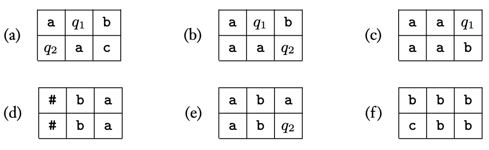
In this figure, windows (a) and (b) are legal because the transition function specifies these are legal actions (recall that the tape head reads the symbol next to the state in the table). Now window (c) is legal because with appearing on the top right, then the symbol appearing in the bottom right, this was possible if the symbol were to the right of and then moved right (as specified by ). Window (d) is legal because the top and bottom are identical, indicating that the tape head is nowhere near these positions and therefore could not have modified them. Also, it is legal for to be in the left column (they can also appear in the right column, but never in the center column). Window (e) is legal because state might have been to the immediate right of the top row, a may have been read, then the tape head may have moved left and transitioned to state , which is a valid transition under . Finally, window (f) is legal because may be to the immediate left of the first row, read , wrote then moved left, which is valid under .
Now with respect to this transition function, here are examples of illegal windows.
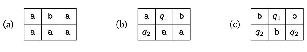
In the above figure, window (a) is illegal since the tape head was not in a position to change to . Window (b) is illegal since the while in state and reading a , the transition function does not allow the machine to write then move left and change to state . Window (c) is illegal because there are two states specified in the bottom row.
Now, intuitively, we want to specify as the formula This says that all possible windows are legal. In the next lecture, we’ll see that this is enough to show the entire Turing machine computation is valid.
-
We switch to the variable here to not conflict with using for the literals of the Boolean formula. In class, I used but the pictures in this section use , so I am re-writing with to keep things consistent. ↩
-
This is slightly different from what was presented in class to make things convenient. ↩
Lecture 5
In-class notes: CS 505 Spring 2025 Lecture 5
Cook-Levin Theorem Wrap-Up
Recall from last time, we are trying to prove that is -complete. To do so, we considered the single-tape non-deterministic Turing machine definition of . Our goal is to show that for any language , we have . That is, is poly-time reducible to .
From last time, we were able to construct an table which encoded the execution of an NTM deciding on input . From this table, we constructed the Boolean formula
The last thing to show is that our definition of correctly captures the correctness of the NTM deciding . Recall that was defined with respect to windows in the table, and it tried to capture the notion of a legal window. That is,
Claim. If the table has a correct starting configuration, and all windows are legal, then is a correct transition from for all .
Proof. To prove the claim, first consider any such . Let and be the and rows of the table. Call the upper configuration and the lower configuration.
Consider all windows for . That is, we look at all windows in the upper and lower configuration. We now define when window is legal. Legal windows fall into two categories: windows which contain a state and those which do not.
-
No state in the window. Suppose window contains no state. Then we say that is legal if and only if the two elements in the center column are equal. The window below is an example. Note that even though in the above example, the first column has then , this would be a legal window because it is possible the tape head is just to the left of in the upper configuration, writes over , then moves left.
-
State in the window. Suppose that window contains a state. Then window is legal if and only if the upper and lower configuration in this window is consistent with the transition function of the Turing machine. In particular, by our construction of the table and since the NTM is a single-tape NTM, a state in the window represents the current position of the tape head. First, we know that when transitioning from the upper configuration to the lower configuration, the state can move at most one position (left, right, or stay). This is easy to check for. Then we know that in the table, the tape head only touches the cell immediately to its right. That is, if the state is in , then the tape head is reading from/writing to . In a nutshell, the computation of a Turing machine is highly local: it can’t jump large distances in a single time-step. Examples of legal windows are given below.
-
Special windows. There are two special windows in any pair of upper and lower configurations: and . These represent the edges of the table. These windows are legal if and only if: (1) they satisfy both of the above constraints; and (2) they have the fixed symbol on the edges. See the examples below.
By the above notion of legal windows, if all windows in the upper and lower configuration are legal, then it represents a correct transition to from . Inductively, this means that if we start with a correct starting configuration, and every window in the table is legal, then each pair of upper and lower configurations represents a valid transition from to , and hence the table correctly captures the computation of the decider for language .
We conclude by giving the Boolean formula for . To do so, we simply need to give a Boolean formula for the statement “.” Define the set as follows. Here, recall that is the cell alphabet of our table.
Given this set , the Boolean formula for the statement “” is expressed as What is this formula saying? It says that given a tuple , which I know by the definition of represents some legal window, is the current window this legal window? That is, it is asking if is true. We take a big OR over all legal windows to make sure that window is some legal window.
If this big OR is true, then we know is some legal window. This gives us the final expression for as All together, we have that is satisfiable if and only if the NTM we are encoding in the table is accepting.
The final piece of the puzzle is arguing that we can construct in polynomial time. Note that the cell alphabet is of constant size with respect to the input length by definition of Turing machines.
- For , given an input to the NTM for deciding the language , the starting configuration of the machine is fixed. Thus, the starting row of the table is fixed as well. For , the starting row of the table contains cells, which corresponds to literals in . This can clearly be constructed in time.
- For , recall that we are simply scanning the entire table for an accepting state. The table has total size , so this formula clearly has size and can be constructed in time.
- For , it is a big AND of pairs . Within this big AND, we have two constant sized subformulas. First, the formula checking that cell contains a valid symbol . Since is constant, the size of this formula is constant. Then this subformula is AND’d with a big AND of an OR which checks that cell doesn’t contain both symbol and . Again, since is constant, this subformula is constant. So the total size of is and can be constructed in this much time as well.
- Similarly, for , the size of the set is at most , which is constant size (something like ) since and are constants. So the inner formula is a constant size, whereas the whole formula is a big AND of pairs from to at most . So has size and can be constructed in this much time.
This completes the proof of the Cook-Levin theorem.
Other NP-Complete Problems
SAT is a step-up from the (useless) -Complete problem TMSAT. However, a general Boolean formula (like those given in SAT) may be difficult to handle when trying to understand specific problems. Thus, we turn our attention to the wide variety of other -complete problems.
First, we show that given any -complete problem/language, if we want to show some other language is -complete, we only need to reduce our known -complete language to our new language.
Theorem 5.1. If is an -complete language, and such that , then is -complete.
Proof. Recall the transitive property of polynomial-time reducible languages. Let be languages such that and . Then we know that .
By our assumption, is -complete. This means that and for all . By our other assumption, we know that . By the transitive property above, we now know that for any . Thus, is -complete.
Now, rather than having to do a complete Cook-Levin Theorem style proof for new languages we want to show are -complete, it suffices to just reduce from a language we know is -complete!
3SAT
We turn to our next (and possibly favorite) -complete language: 3SAT. First, we need to set up some terminology.
Let be a Boolean formula. We say that is in conjunctive normal form (or is a CNF formula) if such that only contains ORs of literals/variables (and their negations). We call each a clause of . One example of a CNF formula with clauses is given below.
We say that is a -CNF formula if each clause contains exactly literals. An example of a -CNF formula with clauses is given below.
Definition (3SAT). The language is the set of all satisfiable -CNF formulas. That is,
Complexity theorists prefer over other NP-complete languages since it is simple, has very little combinatorial structure, and occurs in many differnt contexts such as constraint satisfaction problems.
The other part of the Cook-Levin Theorem (that I hid from you earlier) is that is NP-complete.
Theorem (Cook-Levin, Part 2). is -complete.
Proof. is immediate. What remains to be shown is that is NP-hard. We could show that using our above theorem, but it is actually simpler just to modify the proof of the Cook-Levin theorem directly to give us a 3-CNF formula.
Recall from the proof of the Cook-Levin theorem. First, we will change slightly so that it is a CNF formula (we are almost there already). Once we have put in CNF form, we will then transform it into a -CNF formula.
Since is the AND of clauses, we just need to make sure that each of these clauses is an OR of 1 or more literals. First consider . Recall that it was simply ANDing literals together: So is already a CNF formula with clauses of single literals (there are no ORs).
Now consider . Remember that this is simply a big OR over the entire table, checking if there is at least one accepting state. So will be a single clause of our CNF formula.
Now consider . From before, this is given by Notice that is already in CNF form. The big OR over is a single clause, which gets AND’d with the formula , which is itself a CNF formula. Then all of these formulas are AND’d together, meaning the final formula is in CNF form.
Finally, for , it is a big AND of a big OR of a constant number of ANDs (6 ANDs). Using Boolean equivalences, we can convert the inner formula 1 into a new formula where it is a big AND of some (again constant) number of ORs. This conversion increases the formula size by at most a polynomial-time factor, so is still of polynomial size. All together, this transforms into CNF form in polynomial time.
This together establishes that we can convert our original formula into an equivalent CNF formula, say for some such that each is the OR of one or more literals. We now convert into a -CNF. This can be done as follows. For any , consider the clause .
- If has 3 literals, we are done and can move on to the next clause.
- If has less than 3 literals, we transform it into an equivalent formula with exactly 3 literals. For example, if has one literal, say , we simply write . If has two literals, say and , we pick one of the literals arbitrarily (e.g., always pick the first one) and repeat it, giving . Clearly and are equivalent.
- If has more than 3 literals, we will split into a -CNF formula using extra variables.
For example, if , we introduce the variable and convert to formula
This conversion has the property that if has a satisfying assignment, then there exists an assignment to the variable such that is also satisfied by plus the assignment for .
In our above example, the vector is a satisfying assignment for , and so a satisfying assignment for would be (set ).
In general, if has literals, we introduce new variable and transform into a 3CNF formula with clauses. If has literals , then we construct as Clearly, can be constructed in polynomial time from .
All together, this gives us our new 3CNF formula that is equivalent to the formula we constructed in the Cook-Levin Theorem.
Independent Set
The independent set problem on an undirected graph asks if there exists a set of node/vertices of size at least such that they are pairwise disconnected. That is, for every , . As a set, this is written as
Theorem. is NP-complete.
Proof. Clearly . To see this, one can simply specify a set of size at least . Then, verification that is an independent set takes at most time per pair of since in the worst case you must scan the entire set per check. So the total time is at most in the worst case, where .
Now we show that is NP-complete. We do this by giving a reduction from . That is, .
Suppose that is a 3CNF formula with clauses: . Assume that has literals (note their negation are also literals). For each clause , write , where are the literals of clause . (For example, if , then , , and .)
For each clause , we create a cluster of nodes/vertices in a graph . Label each vertex in this cluster with , , . This gives us clusters of nodes each, where each cluster of nodes is associated with and labeled .
Now we connect nodes in this graph with vertices. First, create a triangle in each cluster. That is, for each , connect , , and (note the graph is undirected so , and are also edges). Next, we connect each node with its negation. For example, if and , then we add the edge to the graph. We claim that the given 3CNF is satisfiable if and only if our constructed graph above has an independent set of size .
First, suppose that has a satisfying assignment. Let be the satisfying assignment. That is, is our satisfying assignment for . From , we build a -independent set in the graph . Now since is satisfied, the assignment satisfies every clause of . Since every clause is satisfied, as least one of its literals , , or is equal to . For each literal , choose only one of its satisfied literals and add it to the set . For example, if , , and under assignment , then add or to (but not both; simply choose one of them).
We claim this set constructed in this manner is an independent set of size . First, suppose that a literal for some (e.g., ). By construction of the graph , we know that is connected to both and . But by our selection of the set , we only choose a single node from each cluster to add to the set. So . Now what if literals for ? By construction of , we know that and are connected if and only if is the negation of the literal represented by . For example, and would be connected in the graph. However, by assumption, the assignment is a satisfying assignment. This means that if were satisfied (i.e, ), then would not be satisfied (i.e., ). So every element satisfies the property that . Thus, is an independent set of size .
Now suppose that our constructed graph has an independent set of size . We reconstruct a satisfying assignment for the formula . Let be the -independent set. Then for every , we know that . We construct our satisfying assignment directly from the set . Suppose . Then set literal in to be . For example if , then we set in the satisfying assignment (that is, ). We claim this is a satisfying assignment. This is by construction of the graph .
- Suppose and is in cluster . Then we know is connected to every other node in its cluster ( are all connected in cluster ). So we know that the other nodes in this cluster are not in (otherwise it would not be an independent set).
- Let such that is in cluster and is in cluster . We know that are not connected. This implies that and are not a literal and their negation (e.g., and is not possible). This means that we don’t obtain an assignment which sets both a literal and its negation to .
Thus, our constructed assignment is satisfying. This completes the proof.
-
Please see the actual definition of for the correct formula here. I am just using a shorthand for demonstration. ↩
Lecture 6
In-class notes: CS 505 Spring 2025 Lecture 6
Brief Aside on Reductions
When we say that a language is polynomial-time reducible to a language , denoted as , we are saying the following.
Given ANY string , I can transform into SOME in polynomial time such that
Looking back at our proof that is NP-complete, we showed how to transform ANY 3CNF formula into SOME PARTICULAR graph such that was satisfiable if and only if has an independent set of size . This is NOT saying that given ANY graph , I can solve ANY 3CNF formula.
More NP-Complete Problems
We’ll show one more problem is NP-complete. Given an undirected graph , a -clique is a set of vertices such that and , we have .1 Let be the set of all graphs that have a -clique.
Theorem. is NP-complete.
Proof. Again, is immediate.
To show that is NP-hard, we reduce 3SAT to . That is, we show . As with , let be a 3CNF formula. Given , we construct a graph with vertices as follows. Label each literal of each clause as , so . For each clause , add a cluster of nodes to the graph with labels . So we have clusters of nodes, where cluster has nodes .
We now add edges to the graph . The graph will have every node connected with edge , except for the following.
- Nodes , , and in cluster (corresponding to ) will not be connected to each other.
- If node is in cluster and node is in cluster , we do not connect and if they are a literal and their negation. For example, if and , then we do not connect the nodes. We argue this graph has a -clique if and only if is satisfiable.
First assume that has a satisfying assignment. Assume has literals and let be the satisfying assignment. Now, we construct a -clique in using the satisfying assignment . Since is satisfying, there is at least one literal in each that has a satisfied variable. For example, in , we can have under the assignment .
For each clause , pick one of the literals that is satisfied by . Suppose this is . Then, add the node in the graph to the set . Repeat this process for all for . Clearly . Now, we claim that is a -clique. By construction of the graph , we know that
- All clusters of nodes are not connected to each other; and
- Nodes corresponding to labels and are not connected to each other; and
- All other nodes are connected to each other. This implies that every node is connected to every other node , so it is a -clique.
Now, assume that has a -clique, denoted by . We construct a satisfying assignment for using . Again, by our construction, we know that:
- All clusters of nodes are not connected to each other; and
- Nodes corresponding to labels and are not connected to each other; and
- All other nodes are connected to each other. Since is a -clique, we know that and for all , we have . We know that and cannot correspond to conflicting variables (i.e., and is not possible if both ). So to construct the satisfying assignment for , for any , we assign the literal correspoding to a . Again by our construction of the graph , we know that each cluster of nodes corresponding to the clause are not connected to each other, but they are connected to everything else. So we know contains exactly node from each cluster of nodes. Thus, we have created an assignment which satisfies all clauses. This completes the proof.
Search vs. Decision Problems
We’ve stated complexity classes as decision problems, but one may naturally consider search variants where we are asked to find solutions. For the class , these two notions are the same: if I can decide a problem, then I can search for an actual solution (and vice versa).
If , then we cannot efficiently search for solutions (i.e, certificates) for decision problems in . On the other hand, if , then we can.
Theorem. If , then for every with efficient deterministic verifier , there exists a polynomial-time deterministic machine such that for all , and .
Proof. We show this is true for SAT, which implies it holds for all of NP since SAT is NP-complete. Suppose that is a decider for . That is, if is a Boolean formula, then if and only if is satisfiable. Since , we know that is deterministic and runs in polynomial time.
Now we build a new machine which outputs a satisfying assignment for if . Suppose that has literals . The algorithm operate as follows.
- On input , the machine :
- Runs .
- If , output reject.
- Else if , we know has a satisfying assignment.
- Set and set (the empty string).
- For :
- Let and be the Boolean formulas obtained by setting literal in to and , respectively.
- Compute and .
- If then set and .
- Else if then set and .
- Output .
Clearly, since runs in polynomial time, then runs in polynomial time (in the length of ). By our construction, if is satisfiable, then the machine correctly reconstructs a satisfying assignment. In particular, during every step of the for loop, at least one of or will be equal to . If not, then the original formula would not be satisfiable, which means we would have already rejected.
The Complexity Class coNP
We’ll now discuss the co-class to NP, which we call coNP. This is defined by the set of languages with complements in NP. That is,
In fact, we know that .
Theorem. .
At a high level, this theorem follows since if , then .
Alternative view of coNP
The above definition of coNP isn’t very useful for understanding what languages in the class look like. So we consider the following equivalent definition.
Definition (). We say a language if there exists a polynomial and a polynomial-time deterministic Turing machine such that
Notice this is the opposite of NP! In the similar definition of NP, we have a “there exists” () rather than the “for all” () in the above definition.
Theorem. If , then . Or, equivalently stated, if , then .
In general, we do not believe that .
coNP-complete Problems
Just like with the NP, we can equivalently define coNP-complete problems. A language is coNP-complete if and for all .
We’ll look at the following problem: deciding if a formula is a tautology. That is, every assignment of variables in is a satisfying assignment.
Theorem. is coNP-complete.
Proof. Clearly since we can build a machine such that for any , and any assignment of variables , if and only if is satisfied. By definition of coNP, this machine must output for all assignments , which is true if is a tautology.
Now we show that is coNP-hard. Let be any language. Consider , its complement language that is in NP (which follows by definition of coNP).
By the Cook-Levin theorem, let be the formula such that is satisfiable, for any . Then, we know Thus, every is polynomial-time reducible to .
The Complexity Class NEXP
Recall the definition of EXP:
We can equivalently define the class of languages decidable in non-deterministic exponential time: NEXP.
Given this, we have a DTIME/NTIME hierarchy of classes:
Perhaps surprisingly, we get a “collapse” if .
Theorem. If , then . Or, equivalently stated, if , then .
-
Note this is the opposite of a -independent set. ↩
Lecture 7
In-class notes: CS 505 Spring 2025 Lecture 7
Diagonalization
Suppose we are given complexity classes and . How can we show they are different? That is, show .
We’ve seen the technique of diagonalization before when we showed undecidability of certain languages. Diagonalization is a general technique that gives us one way of showing the above result: differentiating between complexity classes. Intuitively, if we are given and , diagonalization allows us to differentiate between and as follows.
- If decides , then we want to say is different from any decider for .
- We do this by arguing for any , if then , and vice versa.
Origins of Diagonalization
Diagonalization was originally introduced by Georg Cantor. He used diagonalization to prove that . That is, the set of all natural numbers is strictly smaller than the set of all real numbers. This result at the time was not well received: these are both infinite sets, how could you possibly reason about them being different sizes?
This proof first relies on defining when two infinite-sized sets are the same size. Briefly, two sets of infinite size are said to have the same size if there exists a bijection from to . That is, for every , there is a unique such that .
For example, we know that via the following bijection.
Under this definition of set equality, Cantor showed that . We’ll do an easier proof by showing is smaller than the entire interval of real numbers .
Theorem. .
Proof. We do a proof by contradiction. Suppose that . This means there is a bijection from to . We can write the bijection as an infinite table.
From this table, we’ll construct a new real number that is not in the above bijection. We construct the real number digit by digit. We’ll index digits in the right column of the table starting with (i.e., the first digit after the decimal point is the 0-th digit). Let denote the bijection described by the table.
Then, for each , we define for any such that . That is, the -th digit of will be explicit different from the -th digit of the real number . As a picture, we look at the digits in the table on the diagonal.
Taking the positions on the diagonal, we construct the new real number . Now, there does not exist any such that . This is because for every , we have , which implies that . Thus, the mapping cannot exist.
Time Hierarchies
With diagonalization fleshed out more, we can now discuss time hierarchies.
Deterministic Time Hierarchy
First, we’ll show a time hierarchy theorem for deterministic computations.
Theorem. Let and be time constructible functions such that . Then .
As a corollary of the above theorem, we have:
Corollary. There exists a language decidable in time but not decidable in time for any time constructible function .
We now prove the time hierarchy theorem.
Proof. As you might expect from the preceding discussion, we’ll have a diagonalization proof. First, we build a deterministic Turing machine as follows.
For any and for any , does the following.
- Compute .
- Simulate .
- If halts within steps, output .
- Else output .
Note that step (1) can be done in time since is time constructible. If runs in time , then step (2) runs in time since we can do universal simulation with only logarithmic overhead.
Now, let denote the language of ; i.e., . By definition, decides Moreover, since only simulates for at most steps.
Claim. .
This is where our diagonalization comes into play. Suppose this claim is not true. This implies , and there is a decider deciding in time .
Now, consider running . Suppose that . Then, simulates for at most steps. Notice that runs in time on any input. In particular, runs in time . By universal simulation, we know that simulates in time . Since we have that halts in at most steps. So, for large enough ,1 runs for less than steps. Moreover, by universal simulation, still runs in at most steps on this input.
This implies that completes the simulation of and outputs . However, this implies that . We assumed that decides the language , which also decides by definition, but these two machines differ on this input. This is a contradiction, so does not exist.
We have two important corollaries from the time hierarchy theorem.
Corollary. For all , we have .
Corollary. .
Non-deterministic Time Hierarchy
Now, we move on to show the non-deterministic time hierarchy theorem.
Theorem. Let be time constructible functions such that . Then, .
Proof. Unfortunately, we cannot do a standard diagonalization here. With the deterministic time hierarchy, we simulated the machine (which shouldn’t have existed), and were able to flip its output. The simulation was deterministic and always output the opposite of the machine . However, with non-deterministic simulation, there could be exponentially many outputs on a single input. Recall that a non-deterministic decider needs to only output accept on at least one computation path, and reject on all (when rejecting a string).
The idea behind the non-deterministic simulation will be to do a lazy simulation. In particular, our diagonalization will only differ on a single output; for all other outputs, we will output the correct bit (of the machine we are simulating). This will be enough to derive our contradiction.
We proceed with the proof. Let and let denote the machine described by . Now let be a function such that , , and . Let be any function such that .
Build a non-deterministic Turing machine which does the following. takes as inputs strings of the form for any , where denotes the string of 1’s.
- Compute such that .
- If :
- Non-deterministically simulate for at most steps.
- If halts within steps, output .
- Else output .
- If :
- Deterministically simulate by trying all computation paths.
- Output .
Now, we argue that runs in time . First, step (1) takes at most time. Second, all of step (2) only takes time. Third, step (3.1) takes at most time, which overall takes time. Therefore, runs in time .
Let . By the above discussion, we know that .
Claim. .
Again, suppose this is not the case. Then there is an NTM which decides in at most time. Let be large enough such that for satisfying , we have .
Now, run . If , then simulates for at most steps. By construction, , and runs in non-deterministic time . So the simulation halts before steps and .
This implies the following equalities.
Moreover, by assumption, and both decide the same language . This implies for all , we have This actually shows that for all ; similarly, the same is true for : for all .
Now suppose that . By construction, now simulates deterministically and outputs . Here, outputs if there exists an accepting path, and outputs otherwise. This implies that . But this is a contradiction since above we established that for all . Thus, cannot exist.
-
Recall that every Turing machine has an infinite number of equivalent strings which describe said machine. ↩
Lecture 8
In-class notes: CS 505 Spring 2025 Lecture 8
NP-Intermediate Languages
So far, we’ve looked at many NP problems that also happen to be NP-complete. Thus, it is a natural question to ask whether all languages in NP are NP-complete. It turns out, under the widely believed conjecture that .
Theorem. If , then there exists such that is not NP-complete.
In other words: if all languages are NP-complete, then .
Two examples of languages we believe to not be NP complete are factoring and graph isomorphism. Factoring asks if an integer has prime factors , and graph isomorphism asks if two graphs are isomorphic. This means that there exists a permutation such that for two graphs , if , then .
Oracle Machines
When we showed , we utilized diagonalization. In the proof, we had a decider for some language , and by contradiciton, we assumed we had a machine which decided in time . In the machine , we received as input and simulated it.
At a high-level, diagonalization is possible because of two key properties.
- Turing machines always have efficient representations as strings.
- The universal simulation of any Turing machine given its efficient representation as a bit string does not examine the inner workings of the machine.
In the machines and above, the machine simulates obliviously: it does not even need to look at what is doing, it does not care about the internal mechanisms of . Thus, is treating as a black-box: it gives some input and gives some output.
Oracle Turing Machines
We can abstract these two properties and define oracle Turing machines. These are special Turing machines with an additional oracle tape, and access to some oracle . We denote this as . The machine can query for any input in a single computation step, and writes the output to the special oracle tape in this single computation step.
For a language , we let denote an oracle Turing machine with an oracle to a decider for the language . This allows us to define oracle complexity classes.
- is the set of all languages decidable in deterministic polynomial time relative to the oracle/language .
- is the set of all languages decidable in non-deterministic polynomial time relative to the oracle/language .
As a concrete example, is the set of all languages decidable by a deterministic polynomial-time oracle Turing machine with oracle access to a decider for SAT. That is, if and only if is a satisfiable formula. Recall the complement language of SAT: is the set of all unsatisfiable formula .
Lemma. .
Proof. We build a deterministic polynomial time Turing machine that is given oracle access to such that if and only if is not satisfiable. The machine is simple. On input , queries and outputs the opposite answer. Since if and only if is satisfiable, clearly decides . Moreover, this is polynomial time.
Actually, we can show a stronger result.
Lemma. for any NP-complete language .
At a high-level, given a formula as input, we simply perform a polynomial-time reduction from to the language . For example, we can reduce to a instance, then reduce the instance to (or simply do a direct reduction).
As another result, we know that oracles in do not grant us more power for languages in .
Theorem. For any , we have .
Proof. is immediate since every language in is decidable in polynomial time without an oracle. For , since , we can convert any polynomial time Turing machine with oracle access to to another Turing machine which decides the same language but simply simulates . This simulation is polynomial time, so the final time is polynomial.
Note there are powerful oracles for which and are equal relative to this oracle. One such oracle is for the language , which we define as the set of all tuples where within steps.
Lemma. .
Proof. First, is immediate since any machine with oracle access to can check if an exponential time Turing machine outputs in at most steps. So an exponential time computation can be done in constant time.
Second, is trivially true since .
Third, we show that . Suppose that and is decidable on NTM in time . We construct machine that decides in at most time. is given the description of and deterministically simulates on any input by simulating all possible computation paths. outputs accept if and only if there is at least one accepting computation path, and outputs reject otherwise. Since runs in non-deterministic time , this simulation takes at most time. Finally, whenever calls the oracle on input for some , the machine simply runs the machine for at most steps and returns the result.
Limits of Diagonalization
Oracle machines help us quantify the limits of diagonalization. Diagonalization is quite a powerful, and general technique, so naturally we’d like to resolve vs. using it. Unfortunately, this is impossible.
Theorem. There exists oracle and such that
- ; and
- .
Proof. Setting (the oracle), we have (1) of the theorem by our previous lemma.
Now we construct an oracle to prove (2). Interestingly enough, we will use diagonalization to construct this oracle. First, let be any language. Define a new language as
Notice that for any language . To see this, define machine which (1) guesses ; (2) outputs oracle query . By definition, if and only if ; otherwise it outputs . Clearly, this non-deterministic machine decides .
Now, we construct a new language such that . Then, we will set , completing the proof. We’ll define the language inductively, first by setting . We’ll also have two helper sets (i.e., helper variables) and .
- Step 1.
- Let be the deterministic oracle Turing machine defined by the bit string . For simplicity, we assume that runs in time .
- Choose such that .
- Run .
- Whenever queries oracle at string , reply with /reject. Update .
- If :
- Update . That is, add all -bit strings to the set . Here, is representing the set of all strings that are not in .
- If :
- Find such that .
- Update .
- Update .
- For :
- Assume machine runs in time for inputs of length .
- Choose such that .
- Run .
- Whenever queries oracle at string , update .
- If , reply /reject.
- If , reply /accept.
- If
- Update .
- If
- Find such that .
- Update .
- Update .
Now, we claim that for this language , we have . First, clearly since an NTM can simply guess a correct string in the language . Now, let be any deterministic oracle Turing machine and suppose by way of contradiction that decides . Notice that for each , there are an infinite number of equivalent descriptions for . In particular, there exists some such that . Now, consider . If , it is saying that there exists such that . However, in this case, by construction of (and, in particular, step 2.4.1), we know that all strings of length are in the set and are not in the set . So should output in this case. Similarly, if , then by construction of , we know there exists some length string , so should output in this case. Both cases lead to a contradiction, so .
Intuitively, in the above diagonalization proof, we are exploiting two key facts: (1) there are an infinite number of equivalent Turing machine descriptions; and (2) deterministic Turing machines cannot search an exponential space in polynomial time. (1) allows us to say that if we are given some decider, then there is some for which is the same machine, which means we have considered it in our construction of . (2) allows us to diagonalize. In particular, must produce an output by only making a polynomial number of queries (at most ). Since for large enough , we know that could not have possibly queried the entire set of length bit strings. So, intuitively, the deterministic machine is making a decision with incomplete information.
We exploit this. If , we declare all length strings to not be in the language. Since could not have queried all length strings before outputting its decision, the lack of information leads it to make a wrong decision. Similarly, if , then again there is no way could have queries all length bit strings. So we explicitly find one that was not queried and add it to the set . This again causes to output erroneously. Thus, we cannot decide the language in deterministic polynomial time when given an oracle to .
Lecture 9
In-class notes: CS 505 Spring 2025 Lecture 9
Space Complexity
So far, we have only focused on the time complexity of computations. However, an equally important metric to consider is space complexity. Intuitively, though we would like computations to be fast, time is an abundant resource. For example, we do not need to get new hardware to let computations run longer, we simply just let our computers run longer. However, for space, we cannot simply “download more RAM” or disk space. So it is an important factor to consider in computational complexity.
Definition. Let . A language is in the class if there exists a deterministic Turing machine which decides the language using at most additional space. That is, for any , if and only if and uses space on its non-output work tapes.
Intuitively, when considering the space constraints of an algorithm, we do not count the input length against the space usage (since it must read all the input to do a deterministic computation). We also do not count the output tape (and, in fact, sometimes we remove the output tape and simply encode accept/reject in the final halting state).
Similarly, we define the class as the set of all languages decidable by a non-deterministic Turing machine using at most space on its work tapes for any non-deterministic computational path made by the NTM.
Power of Space-bounded Computations
Intuitively, we believe space-bounded computations to be more powerful than time-bounded ones. This is because we cannot reuse time, but we can continually reuse space. As an example, recall that we do not believe ; that is, no polynomial-time algorithm solves/decides . However, : it is solvable only using linear space by a deterministic Turing machine.
To see this, let be a DTM which takes as input a SAT formula . To decide if (i.e., is satisfiable), we can use linear space and simply test all possible assignments. Suppose that has variables .
:
- For all
- Test if .
- If yes, output .
- Output .
Note we are only keeping track of bits (i.e., we are counting from to in binary) and testing if this produces a satisfying assignment. Testing if is satisfiable under assignment requires space, where , and clearly . Therefore, we only need linear space to decide if is satisfiable. Notably, this is an exponential time algorithm, but only uses linear space.
Space Constructible Functions
Like with time complexity, for space complexity we care about the notion of space constructible functions. As you may guess, these are functions that are constructible in limited space.
Definition. A function such that is space constructible if there exists a deterministic Turing machine such that on input , outputs using at most space on any of its work tapes.
Theorem. For every space constructible function , we have
Proof. Clearly since any deterministic Turing machine running in time can use at most space on its work tapes. Similarly, since every deterministic computation is also a non-deterministic computation.
What remains to show is . To see this, we use the notion of a configuration graph. We let denote the configuration graph of for any NTM . The graph is a directed acyclic graph which consists of all possible configurations of the tape(s) of . There is a unique starting node, which corresponds to the unique starting configuration of every Turing machine. There is an edge from node to in the graph if the configuration can be reached by a valid transition from the configuration in a single step of the computation.
The graph is said to be accepting if there exists a path from the starting configuration to some halting configuration that is accepting. Moreover, if such a path exists, then accepts. One final thing we need is the following fact.
Fact. Any NTM running in time can be converted to an equivalent NTM where the transition function of outputs at most two states per computation step and runs in time .
By definition, we know that the non-deterministic Turing machine transition function is defined as By definition, for a fixed Turing machine , all of , , and are fixed. So . Given this, there is a way to convert the machine with transition function to an equivalent machine with transition function where outputs at most configurations per input.
All together, this allows us to notice the following properties about the configuration graph . If uses space on any input, then
- has at most vertices. In particular, every vertex/configuration can be encoded with space (or for a -tape machine, but is considered constant).
- There exists a CNF of size such that if and only if and are valid configuration sand ; that is, is reachable from in a single step of the computation.
(1) above follows from the above Fact and subsequent discussion. (2) follows directly from the Cook-Levin theorem. In particular, the formula is simply the formula which is checking that all computation windows are valid, and all symbols are valid.
With all of this setup, let be an NTM which decides some language . We construct a machine which decides in time. On input , the machine construct the graph , which takes time. Construction of this graph requires checking edges between nodes, which is done in time per pair of vertices since has size . This gives a total time of . Then simply searches for a path from the starting configuration to an accepting configuration, again taking at most time.
Space Hierarchies
Unsurprisingly, just like with time constructible functions, we have similar space hierarchy theorems for space constructible functions.
Theorem. Let be space constructible functions such that . Then .
The proof is identical to the deterministic time hierarchy theorem, except we do not have the logarithmic loss. This is because of universal simulation: when simulating a time Turing machine, we need time, but to simulate a space Turing machine, we only need space.
Space Complexity Classes
Just like with time complexity, we have complexity classes related to space bounded computations. Four of them will be of interest to us.
- .
- This is the space analogue of .
- .
- This is the space analogue of .
- .
- .
Some facts about the above classes.
- It is an open question of . We believe it to not be true; that is, .
- In a somewhat surprising result, .
- In an even more surprising result, .
We’ll get to the bottom two points in our later discussions on space complexity. Let’s see some examples now.
Space Complexity Class Examples
This implies that . We can see this since for any language , under the certificate definition there exists a DTM and a polynomial such that for all , we have if and only if there exists a string such that . We can easily construct a polynomial space DTM which on input simply iterates over all possible strings and checks if . This only uses polynomial space since we can reuse the space for the string .
Languages in
Checking if a string has an even number of ’s is in , and so is checking if the product of two integers is equal to a third integer. Formally, let
The language is decidable in only logarithmic space because if is the size of the input, counting the number of ’s in only takes bits, then checking if this is even simply requires checking if the least significant bit is . This only takes logarithmic space.
For , we are given the binary representation of three integers , , and . Assume each integer is bits. So the input is of length . Then, to multiply and , one can simply do the grade school multiplication algorithm over the binary representations of and . If we are not careful and try to write down the result of , we would require -bits since is also bits. So we can simply compute bit by bit and compare to the bits of . We will have to track carry over bits, which will be at most bits to track.
Languages in
Deciding if a directed graph has a path between two vertices and is in . Formally, let be the following language. The number of vertices in is and the number of edges is at most . To see that , we give a non-deterministic Turing machine which decides using space. Notice that if there exists a path from to in , then it is of length at most . Thus, a non-deterministic Turing machine simply performs a depth first search of depth at most starting at . If it finds , then it outputs accept; otherwise it outputs reject. If there is a path from to , then there exists a series of non-deterministic choices to make for the depth first search that will end up at .
-complete Languages
We continue our study of space complexity by examining -complete languages. Just like with -complete languages, we define -completeness with respect to polynomial time reductions.
Definition. A language is -complete if
- ; and
- , we have .
True Quantified Boolean Formulas
Up to now, we have only seen “fixed” Boolean formulas. For example, . Then, we say that if and only if such that .
We can generalize the above to include different quantifiers. For example:
- ;
- (notice this is the language , the -complete language);
- .
With this, we can define quantified Boolean formulas.
Definition. Let be a Boolean formula with variables. Then, we say that is a quantified Boolean formula, where and for all . We say that is a true quantified Boolean formula if .
Building on what we have, we let be the set of all true quantified Boolean formulas .
Theorem. is -complete.
Aside: the Essence of
One can actually think of as the set of two-player games with perfect information such that player 1 has a winning strategy. In particular, the essence of turns out to be finding optimal strategies for player 1 in a 2 player game with perfect information (that is, no randomness and no hidden information such as a hand in card games). Three concrete examples: Chess, Go, and Tic-Tac-Toe (though for Tic-Tac-Toe you have to phrase it differently since drawing the game is the optimal strategy). Some other subtleties (which we will not get into in this class) that arise here are, for example, finite boards being easy to deal with in , which need to be fixed by making the board a 2D infinite grid.
Proving is -complete
We’ll begin the proof of this theorem, and finish it in next lecture. For now, we’ll show that . Let be a QBF on variables . We let . We construct a decider to check if , with the goal being this decider uses at most space for some polynomial in .
Let be a simple recursive Turing machine which does the following.
:
- If has no quantifiers, output if and output otherwise.
- Else if 1
- Run with and .
- If returns on either of these inputs, return . Else return .
- Else if
- Run with and .
- Return if and only if returns on both these inputs; otherwise return .
First, clearly decides if . In the base case, if has all variable set to a value, then simply checks if is satisfied by the generated assignment. Then, if , returns if and only if assigning or returns true, which is enough since we only need at least one of these to return true. Finally, if , then returns if and only if assigning and both result in a true QBF.
To finish the proof, note we already established we only need space in the base case of the recursion. The recursion depth is , and at every level we are only storing a single variable worth of information, so the final space complexity is . This finishes the first part of the proof; namely, we have shown .
-
This is another QBF with 0 or more quantifiers. ↩
Lecture 10
In-class notes: CS 505 Spring 2025 Lecture 10
is -hard
Last time, we established that . Now, to show is -complete, we show that it is -hard. That is, , we show .
Let be any language in , and let be the decider for . Suppose that for any input of length , uses at most space for , where is a constant. Recall the configuration graph (see Lecture 9) of a Turing machine . We know that the configuration graph has at most nodes, and each configuration requires bits. By the facts we established last lecture about the configuration graph , we know that if and only if there is a path from the starting configuration to an accepting configuration in the graph . Moreover, there exists an sized formula such that if and only if are valid configurations of and follows from under the transition function of .
For our reduction, our goal will be to take and transform it into a QBF such that if and only if . By our above discussion, we will utilize the configuration graph. The idea will be to construct a QBF that is true if and only if there exists a path from the starting state to the accepting state in the configuration graph .
First Attempt. Let be any directed graph. Suppose we consider two vertices and in such that there is a path from to of length at most for some . Then, there must exist another vertex such that there is a path from to of length at most , and a path from to of length at most . If this wasn’t true; that is, there did not exist such a vertex , then any path from to would need to be of length at least .
Let’s try to build a QBF recursively to take advantage of the above ideas. Let ; i.e., the formula for testing adjacent configurations. Our goal will be to construct (the final QBF, where ; that is, log of the number of nodes in the configuration graph ). In particular, we want to have the property that if and only if there exists a path from the starting configuration to an accepting configuration .
There is actually a simple way to define using our fact about paths between vertices of length at most . For any two configurations , define the formula . Here, the formula if and only if there is a path from to of length at most . We build this formula recursively by saying if and only if there exists a vertex/configuration such that there is a path from to of length at most and a path from to of length at most . Recursively, the formula checks this statement. Finally, when the recursion bottoms out, it reduces to checking if two configurations are adjacent.
If we analyze the size of these formulas, notice that by construction. Then, . Recursively, we have . This gives our final formula size at least . So the formula is too big! It requires exponential space.
Insight: Define an Equivalent QBF. Our final formula had exponential size because we were recursively checking two sub-formulas. This doubled the formula length at each recursion. However, we can take advantage of Boolean logic to define a formula that is equivalent to but only requires a single recursive call to the formula . We define the formula first then explain what each component is doing.
First, is still the target vertex we want to check. That is, we still want to check if there is a path from to of length at most and a path from to of length at most . Now, instead of calling twice and taking the and of the results, we introduce the . What is this doing exactly?
Consider the expression with in the square brackets. This expression evaluates to true if and only if and , or and . In the first case, when and , we check if is true. Great! This is exactly one of the checks we want to perform. Then, in the second case, when and , we again perform the check we want: .
Now, what about for all other values of ? Well, recall that for the Boolean function “,” we know that always evaluates to True, no matter what is. So whenever and are not the target pairs of vertices, the expression trivially evaluates to true. This is fine since we are not checking the distance between these arbitrary variables. However, for the variables we explicitly want to check, the expression will be true if and only if evaluates to true. This gives us the formula we want!
To wrap up the proof, we let , where can be any accepting configuration and is the unique starting configuration. Then, is a QBF which evaluates to if and only if there is a path from to some of length at most (in particular, the exact number of vertices). This happens if and only if .
Finally, we analyze the size of the formula . Notice that . Since , we have that , which is polynomial in since is a polynomial in .
Notice in the proof we actually didn’t use the fact that was a deterministic Turing machine. In fact, the above proof holds even if is a non-deterministic Turing machine. Thus, we have actually shown that is -hard. And since is also a language in , we actually showed that is -complete. This shows the two classes are equal.
Theorem. .
This is a somewhat surprising result since we do not believe the same is true for polynomial-time computations; i.e., we do not believe that equals .
Savich’s Theorem
We can actually show something more fine-grained about deterministic space versus non-deterministic space. The following result would equally show that .
Theorem (Savich’s Theorem). For all space constructible functions , we have .
Proof. We will again take advantage of the configuration graph of a Turing machine that we have been using. Let with corresponding NTM using at most additional space on its worktapes. Let be its corresponding configuration graph with at most nodes for any of length . Recall also that if and only if there is a path in from the start configuration to some accepting configuration.
Our goal will be to construct a deterministic Turing machine which decides using space. The machine will operate as follows.
:
- Simulate by traversing the graph .
- Traversal will utilize a recursive procedure which returns if and only if there is a path from node to node of length at most .
- The recursion utilizes the same fact we had in the proof that is -complete. IN particular, if and only if there exists such that and .
- Suppose has nodes for .
For all accepting states , run .
If this procedure outputs , output .
If none of the calls output , output .
- To run this procedure, each recursive call simply runs over all nodes (this requires bits) and checks if and
- if and only if the edge is in .
Notice that the recursive procedure bottoms out after calls. During each call, we store bits for the current vertex being enumerated over. The machine is performing a depth-first search of the graph . At the bottom of the recursion, space is used. Therefore, uses at most space.
Alternate Proof of
We can use Savich’s Theorem as an alternate proof of this result. Recall that Notice that for any space constructible , we have since all deterministic computations are also non-deterministic. By Savich’s Theorem, we have . Finally, all polynomial functions are space constructible. So this implies for all This shows .
-Completeness
Recall that is the set of all languages decidable on an NTM using at most additional space for inputs of length . We showed last lecture that . Today, we’ll see that is the essence of . That is, is -complete, where Note however that we do not know if , though we believe it to not be the case, otherwise .
Before we show that is -complete, we need a new notion of reducibility that is not polynomial-time. Let’s see why this is the case. Suppose . Then, . That is, any two languages are polynomial-time reducible to each other in . Intuitively, this is because and the reduction trivially has more power than problems in or since it is limited to be polynomial-time only and is not restricted on space. So because we can decide using an NTM using at most space, the reduction can simply compute the configuration graph of the NTM deciding on input , decide if , then produce any instance , all in polynomial time.
Therefore, we need to restrict the power of the reductions for completeness in and . This leads us to logspace reductions.
Definition. Let . We say that is (implicitly) logspace computable if there exists a constant such that for all , and the following languages are in .
We can now define logspace reducible.
Definition. Let and be any language. We say that is logspace reducible to , denoted as , if there exists a logspace computable function such that if and only if .
This finally let us define and -completeness.
Definition. We say that a language is -complete (respectively, -complete) if
- (resp., ); and
- (resp., ), we have .
As with polynomial-time reductions, we have a “transitive” property of logspace reductions.
Theorem.
- If and , then .
- If and then .
Part (2) of the above theorem tells us that if then .
is -complete
We can finally prove that is the “essence” of .
Theorem. is -complete.
Proof. We have already shown that . We now have to show that it is -hard. That is, show that for any . Our good friend the configuration graph will help us yet again.
Let and let be the non-deterministic logspace decider for . This means for any , we have if and only if using at most space.
Our logspace reduction will simply construct the configuration graph . That is, on input , the reduction will output the tuple , where is an accepting configuration. Note that for any .
Recall by definition of our configuration graph, we know that if and only if there is a path from to in . This is precisely a problem instance of . Now, we can represent as an adjacency matrix of size . Entry if and only if there is an edge from to in .
Now, we can check this in logspace. Given , there exists a deterministic machine to check of follows from according to ’s transition function. We can do this in space . By our previous discussions on the configuration graph, these configurations need at most space to represent. Thus, we can do this check in space. Therefore, we have that . So this is a valid logspace reduction.
This completes the proof as we have already encoded into the problem on the instance .
Lecture 11
In-class notes: CS 505 Spring 2025 Lecture 11
Certificate Definition of
Just like with , we can define the class using a deterministic Turing machine that takes a certificate as additional input to help verify whether or not a string is in a language . Recall that for both and , the space used by the input tape is not counted towards the overall space complexity, and the input tape is read-only. So it makes sense that a certificate definition of does not count the size of the certificate when restricting the space complexity.
However, we actually need a stronger property to define with respect to certificates. We need one additional special tape, which we call the certificate/witness tape, with the following properties:
- the space used on the certificate tape is not counted against the overall space usage (as the witness could be polynomial in size); and
- The tape is read-once.
Property (2) above turns out to be crucial, as if you allow the machine to read the certificate multiple times (i.e., it is a read-only tape like the input tape), then you actually end up back in the class .
Definition. We say a language is in if there exists a deterministic Turing machine with a special read-once certificate tape and a polynomial such that for all , if and only if there exists such that , where is the input and is on the input (i.e., read-only) tape and is the certificate/witness and is on the special certificate (i.e., read-once) tape, and uses additional space on its read/write work tapes.
Recall that we do not believe that . This is because under the certificate definition of , there needs to exist at least one certificiate such that the deterministic verifier outputs (i.e., for at least one witness ). In contrast, for , the machine has to output for all certificates of polynomial length (i.e., for all ). So, intuitively, says that we can verify exponentially many certificates using a single certificate of polynomial length. Thus, we do not believe this to be the case.
Turning towards , consider the class . Under the certificate definition, again a machine for must output for all polynomial-sized witnesses . So it was not believed to hold that .
However, this was shown to be true! In particular, it was shown that the -complete problem lies in . Recall that is -complete. Under this definition, we have
Theorem. .
Proof. The key insight into the proof is that if we can enumerate all the vertices which are reachable from in the graph , and is not in this set, then we have shown there does not exist a path from to . We’ll build a certificate which verifies the sizes and the contents of the set of vertices which are reachable from . Our certificate will consist of many sub-certificates, which we will use all together to build the final certificate. The main challenges here are (1) the certificate must be read-once, and (2) we must verify the certificate using only logarithmic space.
Let denote the number of vertices in the graph . Moreover, we will uniquely label each vertex using the set . Note that , so our goal is still to construct a certificate of size while using space. First, let . We say that is reachable from in if there exists a path from to . Now, for every , we can define the set to be the set of vertices such that is reachable from in at most steps. Notice by definition we have .
Now, if we can generate a certificate for the set and show that , we are done. This is because the set is the set of all vertices in the graph that are reachable from in at most steps. Since the graph has vertices, if there is a path from to with more than steps, there is another path from to with at most steps.
Building Sub-certificates. We will build a number of sub-certificates that will help us build our final read-once certificate. First, for any and , we give a read-once certificate showing the statement “”. We’ll call this certificate a certificate.
certificate:
- The certificate will consist of vertices .
- Verification of the certificate proceeds as follows.
- Check if . This can be done in logarithmic space since this is just comparing bits.
- For all , check if . Note here that is part of the input and can be read multiple times. This again can be done in logarithmic space since we are just storing a counter for , and comparing two bit strings of length .
- For all , check if . Again, this is easily done in logarithmic space.
- Count up to and check that . This again only needs bits.
Note here that checks (2) and (3) are done at the same time since we are reading the certificate once. The certificate will be used in our final certificate. One main issue is that we need to be able to verify for any that is actually the set of all vertices reachable from in at most steps in the graph . If we do not verify this, then it is trivial to come up with a certificate that when it actually is.
We’ll now build on the ideas of the certificate . In particular, we’ll need two certificates that are more complicated.
- Certificate : this certificate will certify the statement given that . Here, given means that we have already verified this statement to be true.
- Certificate : this certificate will certify that given that . We’ll use the certificate to help us build these two certificates. Note that by definition, we know that , and it does not need to be included. This will serve as our base case for the final certificate, which will be an “inductive” certificate that continuously builds up to showing that and .
certificate: certifying that given .
- Certificate gives us a certificate for verifying for any .
- Let be this certificate.
- We construct a new certificate for the statement . We denote this certificate by . It is defined as Here, we have and for all .
- Given we know that , we can use the certificate to verify that as follows.
- Run the verification procedure on all to certify they are valid (i.e., the verification procedure for ).
- Check that for all .
- Check that for all .
- Check that has exactly certificates.
Again, all of these checks can be arranged so they are executed in a read-once manner, and they all require only bits of space to check.
Before building the certificate , we actually need another helper certificate, which we denote as . This certificate will certify given .
certificate: certifying that given .
- The certificate here will be identical to the certificate for , except for .
- Let such that for all . Also let denote the certificate for for all .
- Let . This is our certificate for .
- To verify , we perform nearly identical checks as with .
- Verify all are valid.
- Check for all .
- Check that and is not a neighbor of for all .
- Exactly certificates are given.
As always, we can rearrange the above checks to execute them in a read-once manner. Now we have the tools we need to construct a certificate for .
certificate: certifying that given .
- Certificate certifies that .
- Certificate certifes that given . We are also given this by our inductive assumption for this certificate.
- We use this assumption plus the above certificates to construct a certificate for .
- We let denote this certificate.
- It will be the concatenation of certificates, one for every vertex: Here,
- We certify as follows.
- Check that the number of certificates is and that these certificates are valid.
- Certify all certificates using the procedure of .
Final Certificate. All together, we have the tools for the final certificate to verify that there is no path from to in the graph . The final certificate will consist of certificates. Here, is a certificate verifying that given . Note that since we are given by definition, the certificate iteratively builds the sets then , up to . Once the final size of the set is certified, the final certificate is a certificate which certifies that given .
The following is a corollary of the proof.
Corollary. For all space constructible functions , we have .
Introduction to the Polynomial Hierarchy
The motivation for studying the Polynomial Hierarchy is quite simple: sometimes, non-determinism is not strong enough to capture a decision problem itself.
First, recall the independent set problem. Consider the following natural modification of the independent set problem, which we call exact independent set.
Another way to rephrase the exact independent set problem is as follows. if and only if an independent set of size in such that other independent sets , .
If we stated this with a Turing machine, it would look like where intuitively is the certificate for the independent set of size and are all other independent sets in (which the machine checks that they have size at most ). Clearly, this is not captured by the certificate definition of , which is equivalent to the NTM definition. So here, non-determinism alone is not enough.
The Class
Before examining the full Polynomial Hierarchy, let’s capture the set of languages that follow the same structure as the exact independent set problem we outlined above. This is the class .
Definition. The class is the set of all languages such that there exists a deterministic Turing machine (the verifier) and a polynomial such that for all , if and only if .
It is helpful to see another example of a language in the class . This is what is known as , and is defined as follows. Here, a DNF formula is a “reverse” CNF: it is a big OR of many ANDs. Stating it again, if DNF of size at most such that , we have (they agree on all possible assignments).
Notice, in fact, that both and are contained in .
Lecture 12
In-class notes: CS 505 Spring 2025 Lecture 12
The Polynomial Hierarchy
Last time, we defined the class . Today, we’ll generalize this class and define the Polynomial Hierarchy.
Definition. For any , the class is the set of all languages such that there exists a deterministic Turing machine deciding and a polynomial such that for all Here, if is odd and if is even.
Given this generalization of , we can define the Polynomial Hierarchy, which we denote as .
Definition. .
Note that we can also define the co-classes of any . These classes are denoted by .
Definition. For any , . Equivalently, if there exists a deterministic Turing machine deciding and a polynomial such that for all Here, if is even and if is odd.
Actually, we also have that . This is due to the following lemma.
Lemma. For all , we have .
Proof. Let . By definition, there exists DTM and polynomial such that for all , we have if and only if where each . To see that , we can add a “dummy” quantifier in front of . We can define a machine which takes as input , ignores , and outputs . This is clearly in . Note the same strategy works for a language and lifting it to .
Properties of
It is widely believed that , , and for all . This is because otherwise, the Polynomial Hierarchy collapses. That is, there exists such that or (which implies that ). We say this is a collapse of because if this happens, the .
Theorem.
- If there exists such that , then .
- If , then .
Proof. Notice that (2) is actually just a corollary of (1) when . However, we’ll directly prove (2), as the ideas in this proof readily extend to any . We’ll do a proof by induction. Suppose that . Recall this also implies that . Our proof by induction will establish that for all .
For the base case, we have that since . For the inductive step, assume that . We show that .
First, we show the case for . Given , by definition we have a DTM which decides . That is, for polynomial and any , if and only if where all .
Define new language to be all pairs such that Clearly, we have that by our inductive hyptophesis. This implies there exists a DTM such that if and only if , where runs in polynomial time. Now, we can replace the decider for with as follows. Under this , we have that if and only if . Now this implies that . Therefore, .
For the other case, where , we simply do the above strategy for the complement language .
Complete Problems for
We can readily define complete problems for , , and , using the same definition of polynomial-time reducibility we have for . And, in fact, for every , and have complete problems.
However, we do not believe that has a complete problem/language . This is because if one were to exist, then again collapses to some level .
Theorem. If there exists that is -complete, then there exists such that .
Proof. Recall that . So for any , there exists such that or . Assume that is -complete. Then, for all , we have . Suppose that . This implies that if or for , we can in polynomial time decide using a decider for . Since , this implies that as well. The same holds if . Thus, collapses to level .
Recall that is the complete problem for . Recalling the definition of , it is a more general quantified Boolean formula and caputres computations in . So we have . However, as a corollary of the above theorem, unless collapses, then is a strict subset of .
Corollary. Unless collapses, .
This is simply because is a complete problem for , so if , then has the complete problem , so it must collapse to some level .
Complete Problems for an and
In contrast to , for any fixed , the classes and each have complete problems.
-
For , we define the language as follows. where if is odd and if is even. Then, is -complete.
-
For , we define the language as follows. where if is even and if is odd. Then, is -complete.
-
A different complete problem for , due to Umans in 1998. This is called . The problem is defined as follows. The input to the problem is a set of DNF formulas each with variables, and an integer . This input is said to be in if and only if there exists a subset of size at most such that the formula is a tautology. More formally, Clearly, this language is in . It turns out it is also -hard.
Alternating Turing Machines: Generalized Non-Determinism
Let’s think back to the non-deterministic Turing machine definition of . We say that if there exists a NTM which decides . This was defined as follows: for all , if and only if , where we say outputs 1 if and only if there is at least one set of non-deterministic choices makes on input that causes to output . Viewing this as a computation tree, or from the point of view of our configuration graph , it says that there is at least one path from to any accepting configuration in . Moreover, all paths to halting configurations have length .
Now, thinking back to , it is reversed: an NTM decides if for any , if and only if in the graph , all halting configurations are accepting. If this happens, we say that ; otherwise, if there is at least one rejecting configuration, .
How can we model this for, say, ? That is, is there a way to describe a non-deterministic machine which decides ? Looking at the deterministic verifier definition, if there exists deterministic verifier such that for all ,
It is not immediately clear how we would define a non-deterministic Turing machine to decide . For languages in , it was enough that there existed at least one accepting configuration in , and for , we needed all halting configurations to be accepting in . Thinking to the verification definitions of , this makes sense. But how can we generalize it to , and more generally and ?
Alternating Turing Machines
The answer is alternating Turing machines. These machines, in some sense, generalize non-determinism as follows.
Definition. A non-determinstic Turing machine is said to be an alternating Turing machine (ATM) if it additionally labels non-halting states with or such that for any , if and only if the starting configuration is labeled after the following process.
- Let be the directed configuration graph for .
- Label all configurations with and with .
- For all non-halting nodes in the graph , corresponding to some non-halting configuration:
- If the state of is labeled , label with a if and only if at least one child of is labeled .
- If the state of is labeled , label with a if and only if all children of are labeled . We say that an ATM runs in time if all root-to-leaf paths in have length at most for any input . Finally, we say that an ATM is -alternating if on any root-to-leaf path in , it alternates between and state label quantifiers at most times.
Under the above definition, it is clear that is decidable in polynomial time on an ATM which is -alternating. That is, the ATM begins only with states, then at some point switches to states, until the computation halts. We can now define alternating time and space.
Definition. For function , we say that if there exists an ATM which decides in at most time. Similarly, for function , we say that if there exists an ATM which decides in at most space.
Lecture 13
In-class notes: CS 505 Spring 2025 Lecture 13
In this lecture, we wrap up our discussion of Alternating Turing machines and the Polynomial Hierarchy.
Alternating Time and Space
Given ATMs from last lecture, we can alternatively define , , and in terms of ATMs.
Definition. The class (resp., ) is the set of all languages that are decidable in time on an -alternating ATM with initial state labeled (resp., ).
It is not difficult to see how we can define and with respect to the above complexity classes.
Lemma. For all ,
Corollary. .
Unlimited Number of Alternations
The definitions above of and limit the number of alternations a given ATM can have (they are -alternating). However, we do not need to restrict the number of alternations. This was exactly the class defined in the last lecture: the set of all languages decidable in time by an ATM . In particular, there is no restriction on the number of alternations. With this, we can define alternating polynomial time.
Definition. .
As one might expect, an unlimited number of alternations yields something we believe to be more powerful than .
Theorem. .
Proof. First, we show that . We do this by showing . Recall that a QBF is in if and only if (i.e., it is a true quantified Boolean formula), where for all . This is trivially sovlable by an ATM which guesses everything and labels states according to , and checks if the result is true in polynomial time.
Now, we show . Let with ATM deciding in polynomial time. Construct a deterministic machine as follows. On input , performs a depth-first search of the configuration graph and attempts to compute the label of the starting node (which would be the output of the machine . The algorithm is recursive. Recalling the facts about the configuration graph, since runs in polynomial time, the amount of bits needed to represent every configuration is polynomial in . Moreover, doing a depth-first search only requires storing configurations in the recursion stack, since runs in time. So uses at most polynomial space.
We can also define alternating polynomial space, where we consider space-bounded ATMs with an unlimited number of alternations (the class .
Definition. .
Theorem. .
Finally, we can define alternating logspace as .
Theorem. .
Time-Space Tradeoffs for SAT
What are alternations used for? Here, we’ll see how we can use ATMs to give time-space tradeoffs for .
Complexity theorists generally believe that any algorithm deciding/solving must have the following properties.
- Solving requires exponential time (or, at least super polynomal time).
- Solving requires linear space.
In general, both of the above are conjectures, there may be an algorithm for solving which only uses logarithmic space, or uses polynomial time! However, we can rule out an algorithm that achieves both of these properties.
Theorem. Let be functions. Define the class to be all languages decidable by a DTM using at most time and (additional) space. Then, . More generally, for any such that , we have .
Proof. To prove the theorem, we first need the following claim which relates to .
Claim 1. .
The proof of this claim is similar to the proofs of Savitch’s Theorem and is complete. Let with decider running in time and space for any input . We construct an ATM for deciding as follows. will construct the configuration graph . By the previous properties we have discussed for configuration graphs, we know that all configurations need at most bits to describe. Moreover, if and only if there exists a path in the graph from to some accepting configuration , and any such path has length at most .
Now, this path from to exists if and only if there exist configurations such that:
- If , then is accepting; and
- , follows from in at most valid executions of ’s transition function. Essentially, we have divided the path from to into chunks, each of size . Now, each configuration requires bits to describe, so the full description of the path requires bits. So the ATM guesses this path using the appropriate alternations. Intuitively, this is is a start state, is an accepting state, and follows from in at most steps. Clearly, this implies .
Now, we need a second claim to proceed with the proof.
Claim 2. Suppose that . Then .
To see this claim, let . Then there exists a DTM such that in time, where . Here, we are using the fact that .
By the assumption in the claim, we have . By a padding argument, this implies that . Thus, we can construct a DTM such that on input for and , runs in time and outputs if and only if such that . This implies that
Why have we bothered with Claims 1 and 2? Well, using these claims, we will show that . This establishes the result since . Suppose this is not the case; that is, . Then, Claims 1 and 2 gives us the following inequalities. where follows by Claim 2 and the fact that . This violates the non-deterministic time hierarchy theorem, so we can conclude that .
The Polynomial Hierarchy via Oracle Machines
Our final discussion on the polynomial hierarchy will again show that we can give yet another equivalent definition, this time using oracle Turing machines/complexity classes. We begin with .
Theorem. For all , we have , where is a -complete problem.
Proof. We show the proof for , other cases are analogous. For , we show that . First, we show . Let . By definition, there exists a DTM such that for all , we have if and only if , where . Fix such that . Now, the language of all pairs satisfying this is a language. To check if , we can equivalently check the statement . That is, we can check if . Since this is a statement, we can check this statement in polynomial time by converting it to a formula and querying the oracle to see if it has a satisfying assignment. Thus and .
Now, we show the other direction: . Let with corresponding NTM . Here, we assume that the NTM outputs at most choices per execution of its transition function. At first glance, it does not seem like we can capture the power of the oracle in . After all, for any , makes at most queries, say (note: each is a formula), each with corresponding answers . Moreover, each query can arbitrarily depend on the previous queires and answers, along with any other non-deterministic decisions made by !
Let denote the non-deterministic choices made by . Intuitively, in order to construct a DTM to decide in , we will guess the non-deterministic choices and query answers that will cause to accept. That is, we can see that if and only if choices and query answers such that
- If makes choices and recieves oracle query answers ,
- Then
- reaches an accepting state and
- The following hold.
- If then there exists an assignment such that .
- If then for all assignments we have . Here, is the th query made by .
Thus, we construct a DTM such that if and only if simulates and
- using non-deterministic choices ;
- :
- If then ; and
- If then .
Clearly, decides and thus .
Lecture 14
In-class notes: CS 505 Spring 2025 Lecture 14
Randomized Computations
So far, we have only examined deterministic and non-deterministic Turing machines. Crucially, neither of these models for Turing machines utilize randomness. This is obvious for deterministic Turing machines, but it is very important to understand that non-determinism is not randomness, it is an idealized computation model that is not realistic.
Today, we’ll consider probabilistic Turing machines. These Turing machines will be allowed to sample uniformly and independently random bits and use these bits to help make decisions. Here, uniformly random means that , and independent means that the probability is or does not depend on any previous bits sampled or decision made by the algorithm.
Definition. A probabilistic Turing machine (PTM) is a Turing machine with two transition functions . For all , a PTM on input does the following.
- For each step of the computation, samples .
- Execute .
We let denote the random variable corresponding to PTM ’s output on input given the random choices it makes during its execution. We say that runs in time if for all , halts in steps for any set of random choices.
Deciding Languages: PTMs vs NTMs
As stated above, PTMs and NTMs are not the same. Recall that for NP, we say that an NTM accepts a string if there exists an execution of such that . Similarly, for coNP, the NTM accepts string if all executions of satisfy . Above, these definitions are quantified with respect to any possible non-deterministic choices the NTM make during its execution.
Now, for a PTM, say , we can similarly define it with respect to the number of accepting paths. That is, we can say that accepts a string if some fraction of all executions satisfy . For example, we can specify that if for at least half of all computation paths (that is, looking at every possible set of computation paths could take using randomness), then we say accepts . This gives us a natural definition for deciding a language with a PTM.
Definition. Let be a language and be a function. We say that a PTM decides in time if halts in time for any and where the probability is taken over the random choices made by on input , and if and if .
In the above definition, decidability with respect to a PTM has two-sided error, meaning that outputs correctly with probability at least for both and . This leads us to our first probabilistic complexity class: BPP.
Definition. For a function , we say that a language if there exists a PTM which decides in time . The complexity class BPP is defined as
Note that BPP is still a worst-case class since we require deciding languages on a PTM in strict polynomial time.
BPP vs. Other Classes
Intuitively, like how NP was the non-deterministic analogue of P, BPP is the randomized analogue of P. In fact, we know that . To see the first inequality, notice that every deterministic algorithm is a randomized algorithm that uses no randomness (e.g., you just pick , where is the transition function of the DTM). For the second inequality, suppose that is a PTM running in time . Then has possible computation paths (each step picks 0/1 with equal probability). So we can construct a machine running in time which enumerates all possible computation paths of and outputs if and only if at least 2/3 of the paths are accepting.
Now, it is unknown whether or if . For the second statement, most complexity theorists actually believe that , but this is a topic we will not cover in this course.
This is not the last time we will see how BPP relates to other classes; we will return to this topic in later lectures.
Alternate Definition of BPP
Taking inspiration from the above outline of , we can give an alternative definition of BPP similar to the certificate definition of NP.
Definition. A language is in the class BPP if there exists a polynomial-time deterministic Turing machine and a polynomial such that for all ,
3 Examples of BPP Algorithms
We’ll now give 3 examples of randomized algorithms.
Finding the Median
Given a set of numbers , the median of is the number such that for elements and for elements . Stated as a decision problem, you’d be given and would need to decide if is the median of .
There is an easy deterministic algorithm that requires time to check.
- Sort and obtain , where for all .
- If is even, set (more generally, any number in the range ). If is odd, set .
This takes time since we sort .
Now there is a time deterministic algorithm for finding the median and, more generally, the th smallest element. However, the algorithm is highly non-trivial.
To contrast, we will give an time simple randomized algorithm to find the th smallest element, where an element is the th smallest if satisfy and satisfy . In particular, setting gives us the median problem. Let .
- FindthElement:
- Pick . Set .
- Scan and let denote the number of elements such that .
- If , output .
- If :
- Create set .
- Run FindthElement.
- If :
- Let .
- Run FindthElement.
We now give the intuition on why this algorithm runs in time for initial list size .
- The deterministic parts of the algorithm run in linear time.
- The expected sizes of and can be shown to be at most . That is, with good/high probability over the random choice of , and (where the “” is updated every recursive call to mean ).
- Together, this implies that if is the runtime of the algorithm, then , which can be shown to imply that .
Polynomial Identity Testing
Polynomial identity testing is very common in many areas of theoretical computer science and cryptography. Consider an variate polynomial with integer coefficients We define the degree of to be , where is the largest degree of in . For example, if , then .
The most natural identity to test is whether is the identically zero polynomial. That is, for all . Note that this isn’t even checkable in polynomial time. One can give a with a small description but, once expanded, contain terms! An example of one such polynomial is for some constants .
However, there is a probabilistic algorithm which can efficiently check if is identically zero, assuming that evaluating at any single point is efficient (i.e., polynomial-time).
:
- Sample .
- Sample uniformly random .
- Check if . Output if this check passes, and otherwise.
Observations. Let .
- If then for any .
- Suppose that . We want to analyze the probability that . This is equal to the probability that divides . Suppose that has prime factors . We can upper bound the probability that divides by the probability that is any one of these prime numbers. By the Prime Number Theorem, the number of primes in is at least . Now, one can show that . This implies that the number of elements of not equal to is at least . So, with probability at least , the randomly chosen will not be equal to any of . This gives us
- Now suppose that but is not the identically zero polynomial. This means that is a root of the polynomial . By the Schwartz-Zippel lemma, this implies that
All together, these observations imply that
Verifying Matrix Multiplications
Let be a prime number and let be the set of integers modulo . Fix three matrices . We want to decide if .
The fastest known matrix multiplication algorithm runs in time (and, I believe, is not possible to be run on a real computer because the hidden constant is enormous). There is also the trivial algorithm which takes time; here, we’re actually counting the number of operations, so this algorithm takes roughly multiplications and additions over .
We can use randomness to get an -time algorithm to verify if . The algorithm operates as follows.
- Sample .
- Create vector .
- Check if . Output if and only if this check passes.
Notice that computing takes time. Similarly, computing takes time, and also takes time, so the algorithm runs in time.
Now, if , then for any choice of , and thus with probability if then . What if ? This basically reduces to polynomial equality checks (or, equivalently, zero-checks). Let be the th row of . Then, if we set , we have that . Recall that , so this inner product looks like , which looks exactly like evaluating a degree polynomial, say , at a random point .
Now, if we set , suppose that in row , we have . Then, our random check is actually testing the following: In particular, the above is true if and differ on a single entry! So this shows that
One-Sided Error
Interestingly, the above algorithms all have stronger guarantees than just BPP gives. Finding the median always outputs the correct answer, but runs in expected linear time. Both polynomial identity testing and verifying matrix multiplications will answer “YES” with probability when the polynomial given as input is identically zero and when for the given matrices, but both of these algorithms will output “YES” with small probability (not equal to ) when the input does not have the correct form.
Building on the latter two algorithms, this lets define two “stronger” classes than BPP which have one-sided error.
Definition. The class is the set of all languages that are decidable by a PTM running in time such that for all We define the class RP as
Naturally, we have the co-class of RP, called coRP defined as . Equivalently, it is also a one-sided error class with the opposite guarantees as RP.
Definition. The class is the set of all languages that are decidable by a PTM running in time such that for all We define the class coRP as
Lecture 15
In-class notes: CS 505 Spring 2025 Lecture 15
Zero-Sided Error
Last time, we discussed BPP, RP, and coRP, which are 3 (worst-case) probabilistic complexity classes.
- BPP is the set of all languages decidable in strict polynomial-time by a PTM such that . BPP is a two-sided error class.
- RP is the set of all languages decidable in (again) strict polynomial-time by a PTM such that implies and implies . RP is a one-sided error class, where it never has false positives (i.e., outputs when the answer is ).
- coRP is the set of all languages decidable in (again) strict polynomial-time by a PTM such that implies and implies . coRP is a one-sided error class, where it never has false negatives (i.e., outputs when the answer is ).
Now we turn to zero-sided error. Intuitively, zero-sided means that a PTM always outputs correctly; that is, . You would be correct in thinking that if this happens in strict polynomial-time, then this class would just be P. So, in order to not have the same class, the probabilistic class of languages decidable with zero-sided error is relaxed to have PTMs that run in expected polynomial time. This is the class ZPP.
Definition. The class is the set of all languages decidable on a PTM running in expected time such that for all . In particular, if is the random variable for the runtime of on input , then if and only if and for all . The class ZPP is the set of all languages decidable in expected polynomial-time with zero-sided error; i.e.,
ZPP vs RP and coRP
Since we have deviated from strict polynomial time to expected polynomial time, one may wonder how ZPP relates to RP and coRP. The following theorem exactly captures this relationship.
Theorem.
Proof. We show both directions. First, we show that . Let . Let be the RP machine and be the coRP machine. In particular, the following hold.
We construct a new PTM which will decide with zero-sided error in expected polynomial time. on input does the following.
-
- While
true:- Run and to completion.
- If they both output (accept), then output (accept).
- If they both output (reject), then output (reject).
- While
First, we show that (eventually) if halts then . Notice that will always halt. This can be seen as follows.
- For ,
- . In particular, we will never have in this case. will run until , which happens with probability at least . In this case . Since the probability is not zero, there is a series of random choices that can make that will make it output , so will halt and output .
- If ,
- . So we have the reverse of above: will never happen. So can only output in this case, and it will do so eventually since in this case.
Now, we argue that runs in expected polynomial time. Let be a polynomial such that and both run in time at most for inputs of length . We analyze the expected running time of on input . Let denote the random variable for the runtime of on input . First, notice that for every iteration of the loop, runs in time at most to run both and to completion, assuming that . So if we are in the th iteration of the loop, at the end of the loop, will have run for steps.1
So to analyze the expected runtime of , we have Now, we analyze . This probability is identical to the probability that halts after the th loop. We analyze this probability, starting with .
-
. In this case, halts after one execution of and . This means after one execution, they are in agreement. For both and , this happens with probability at least . Without loss of generality, through the remainder of the proof we assume that the probability this happens is exactly .
-
. In this case, the first execution of the loop resulted in , and the second execution has . Implicitly, we have assumed that does not reuse randomness in every subsequent execution of the loop, so each run of and are independent of previous runs. Now, the probability that for any is (at most) . So in this case, the probability that halts after loops is equal to .
Extending the above analysis to any gives us This then tells us
where the last equality can be shown using infinite sum tricks. So, we have shown that runs in expected polynomial time . Thus, .
Now for the other (easier) direction, we show that . For this, we will need a result known as Markov’s Inequality.
Markov’s Inequality states that if you have a non-negative random variable , then for any , it holds that We’ll use this inequality to show .
Let be the ZPP PTM that decides . Suppose that decides in expected polynomial time for inputs of length . In particular, if and only if , and runs in expected time for any .
We construct a new PTM which does the following.
-
- Compute .
- Run for at most steps.
- If halts within steps, output whateer outputs.
- Output .
We show that is the RP machine deciding . First, we show that if , then . Notice that if halts within steps, then by definition of ZPP. Then, if does not halt within steps, the machine otuputs . So in either case, and thus .
Now assume that . We need to show that . By definition of , if and only if within steps. In particular, we know that since , so we must show that halts within steps with probability at least .
Let denote the random variable for the runtime of . By definition, . Applying Markov’s inequality, set . Then, we have
This tells us showing that .
Now, to show that , we construct PTM identically to the PTM , except the machine outputs if does not halt within steps. The analysis is identical to the above analysis. Therefore, and thus .
-
Technically speaking, to run and , needs time for universal simulation, but we can simply upper bound this by another polynomial and the analysis remains the same. ↩
Lecture 16
In-class notes: CS 505 Spring 2025 Lecture 16
Error Reduction for BPP
Recall that a language is in BPP if there exists a strict polynomial time probabilistic Turing machine such that for any , . Equivalently stated, for a deterministic Turing machine running in polynomial time, it holds that for all , where .
Here, the error probability is convenient, but arbitrary. We’ll see that the class BPP is equivalently defined for any error probability at least .
Definition. For any , the class is the set of all languages such that there exists a probabilistic Turing machine running in strict polynomial time such that for all , .
Under the above definition, we can set for constant for , or even . We’ll show that this BPP class with reduced error is equivalent to the standard BPP definition.
Theorem. For all constants , it holds that .
Proof. Clearly, since for all and large enough . Next, we show the other direction, namely . We show this via the following claim.
Claim. Suppose is decidable by a PTM (in polynomial time) such that for all , for some constant . Then there exists a PTM running in polynomial time and a constant such that for all , .
We won’t show the full proof, but just the main ideas. The idea is that the machine will simply run for some polynomial number of times, then output the majority of the outputs. Let . Then, will independently run times. Let be the output bits of the independent runs of . Then, outputs , where if of the bits are ; otherwise, . It can be shown using the Chernoff bound that if , then under the parameters we’ve set. Notice also that runs in polynomial time since it runs a polynomial number of times.
With the claim, for large enough , it holds that , which shows that whenever .
BPP vs. Other Classes
Now, we examine the relationship between BPP and other complexity classes.
BPP vs P
First, we naturally ask: what is the relationship between P and BPP? Clearly, since any deterministic Turing machine is also probabilistic (you can either set , or have ignore the random input ). Many complexity theorists actually believe that , which concerns the rich field of derandomization and hardness amplification. But we will not examine these fields in this course.
BPP vs PH
At first glance, it is not clear what the relationship between the polynomial hierarchy and BPP is. It turns out that BPP sits low in the polynomial hierarchy.
Theorem. .
Proof. Note that since , it suffices to show either or . We show that .
Let (which is equivalent to BPP by the previous theorem and claim). Using the DTM definition of BPP, there exists a DTM running in polynomial time such that for all , it holds that , where for some polynomial .
Let for . We define a set as the set of all good strings for . That is, ; i.e., the set of all such that . Otherwise, if , we say that is bad for .
- Notice that if , it holds that . This is because when , and thus there must be at least strings such that .
- If , it holds that . This is because if , then , so there is at most fraction of strings such that .
Now, the goal is to encode the set as a statement. We’ll need the following tool. For any and any vector , define . Now set .
Claim 1. If , then for all , it holds that
Proof of Claim 1. Notice that for any , we have . Then by a simple Union bound, we have
Claim 2. If then there exists such that
Proof of Claim 2. We use the probabilistic method. If we can show that for uniformly and independently sampled , then there must exist vectors such that For , let denote the “bad event” that . We show that .
Consider for any . We show that . Let denote the event that . Equivalently stated, . Notice that .
Now, since is uniformly sampled, we know that is uniformly distributed in . So we know that , which implies that . So . Finally, all are independent, so we have , where the last inequality follows since . This implies again by the Union bound that , which implies that so there exists vectors such that
Now, given the two claims above, we can now decide using a machine as follows. For any , define the machine which operates as follows. outputs if and only if , where . Therefore, if and only if . Thus, .
Randomized Reductions
We can define a slightly weaker notion of reduction than the polynomial time reductions we’ve seen before. We’ll see randomized reductions now.
Definition. For languages , we say that is randomized polynomial-time reducible to , denoted by , if there exists a polynomial time probabilistic Turing machine such that for all , we have .
Note that randomized reductions are not transitive! That is, if and , it is not necessarily the case that . However, randomized reductions are still useful. One can show that if and , then .
NP under Randomized Reductions?
We can define an NP-like class for NP under randomized reductions. This is the class . Note that we can equivalently define as .
Generally speaking, complexity theorists believe that . They also do not believe that because of the following lemma.
Lemma. If , then .
Randomized Space-bounded Computations
We can also examine space-bounded computations through the lens of probabilistic Turing machines. The most interesting space-bounded randomized computations are those which only use logarithmic space.
Definition. The class is the set of all languages such that there exists a strict polynomial-time PTM using additional space for inputs of length at most such that .
BPL is the log-space equivalent of BPP, and we can similarly log-space equivalents of RP, coRP, and ZPP, denoted as RL, coRL, and ZPL.
Theorem.
- .
- .
Boolean Circuits
We will now turn our attention to Boolean circuits, or just circuits. Circuits are inherently a non-uniform model of computation. That is, circuits have a fixed input length, rather than being able to operate over infinitely many input lengths. For example, Turing machines are a uniform computation model, where a single Turing machine takes infinitely many inputs .
Circuits, on the other hand, can only operate over a fixed input length. For example, a circuit computes some function over inputs for a fixed , and every has some different circuit.
Definition. A Boolean circuit of size with -bit inputs is a directed acyclic graph on vertices with the following syntax.
- The input vertices have in-degree and unlimited out-degree.
- The remaining non-input nodes, which we call gates, are all labeled AND, OR, and NOT (corresponding to the Boolean functions AND, OR, NOT) and operate as follows.
- AND and OR gates both have in-degree 2 (or fan-in 2) out-degree 1 (fan-out 1).
- NOT gates have in-degree and out-degree 1.
- There is a single output gate with out-degree 0 (note this gate can be an input node/gate, or any internal node).
Circuit Families
Since circuits are non-uniform, one circuit cannot decide an entire language (unless only contains strings of one fixed length). Thus, we need to define circuit families to handle variable length inputs.
Definition. Let be a function. A -sized circuit family is a sequence of circuits such that and has input gates for all . We say that a language is in the class if there exists an -sized circuit family which decides ; that is, for all and , if and only if .
Examples.
-
The unary language lies within ; that is, . Moreover, any unary language is in .
-
For , we have .
Lecture 17
In-class notes: CS 505 Spring 2025 Lecture 17
Continuing our discussion on circuits, recall that is the set of all languages that are decidable by an -sized circuit family , where for all , we have if and only if .
We highlight two facts related to circuits.
- Any (3)CNF Boolean formula is a special-case of circuits.
- Recall at the beginning of class this semester, we stated that every Boolean function has an sized CNF formula computing it.
This readily implies that any such function is computable by an -sized circuit.
- Shannon improved this bound to for any such .
- Others improved over Shannon, giving an upper bound of .
Circuit Complexity: P/poly
We’ll not discuss what complexity theorists feel is one of the most important circuit complexity classes: . Intuitively, this is the circuit equivalent of .
Definition. The class is the set of all polynomial-sized circuits. That is, .
Theorem. .
Proof. First, recall that any time- Turing machine has an equivalent oblivious Turing machine running in time (in class, we saw a simpler proof of ). The properties of this machine are as follows.
- For all , .
- At any timestep , the position of the tape heads of are a function of and the current timestep (that is, they only depend on these two quantities).
Crucially, (2) above tells us for any fixed input length , the machine for any moves its heads the exact same way. Now, to show the theorem, we will argue that every time- oblivious TM has an -sized circuit family deciding it. The remainder of the proof will be a high-level overview.
Let denote the runtime of . For timestep , we define to be a snapshot of the execution of on input . This snapshot contains
- The current state of at timestep
- All symbols under the tape heads of .
Since for every fixed Turing machine, the number of states and tapes is constant, we have that for every . Now, we define a transcript of as , where is the initial snapshot of in its initial configuration, and snapshot follows from via the transition function. That is, we can write (to abuse notation).
The key observation here is that since each is constant-size, and moving from to for every only depends on and , we can compute each using a constant-sized circuit.
This constant-sized circuit, which we denote by , takes as input and (and assumes that ) and outputs .
Then, to construct the final circuit , we simply compose all of these sub-circuits together to compute , and a final sub-circuit which reads and outputs if and only if contains the accept state.
This circuit has size , and we can define such a circuit for every input length .
Finally, the circuit has worst-case size if we started with a non-oblivious Turing machine.
Note. In the above proof, the transformation from the non-oblivious Turing machine to a circuit can be performed in polynomial-time and logarithmic space. We will use this fact later.
P is a strict subset of P/poly
The non-uniform power of can be showcased in a number of ways. Here, we’ll first show that the inclusion of the above theorem is strict. That is, . This follows from last lecture when we stated that any unary language is in .
Lemma. For any , we have .
Proof. For every , we have two cases. First, if , we define the circuit to be the constant-sized circuit encoding the Boolean formula , ignoring all other input bits.1 This formula always outputs , so it will always reject since (and no other strings of length are in too).
Now, if , we define to be the -size circuit encoding . This formula outputs if and only if .
Why does this show ? It is because we can encode Turing undecidable problems into unary languages. Consider the following unary halting problem language.
Clearly, , so , but is not Turing decidable!
Alternate Proof of Cook-Levin Theorem
We can use circuits and obtain an alternate proof of the Cook-Levin theorem. To do this, we’ll need the language of circuit satisfiablility. We let denote the set of all strings such that encodes a circuit with a -bit output and there exists such that .
Theorem. is NP-complete.
Proof. It is clear that since given the encoding and a string , one can check in time if . Now, we show that is NP-hard. To see this, we must show that for all , we have . Fortunately, in our proof that , the transformation from a Turing machine running in time to a -sized circuit family is (1) a polynomial-time transformation; and (2) works for non-deterministic Turing machines as well. Or, if we strictly use deterministic Turing machines, this proof shows how to transform any polynomial-time verifier (i.e., iff such that ) into a polynomial-sized circuit family such that if and only if such that .
With the above theorem, to show an alternate proof of the Cook-Levin theorem, we must now show that . This is done by constructing a 3CNF formula as follows. Consider any circuit and any node in with parent nodes and .
- If is the AND of and , we encode the Boolean formula “” in the formula , using the fact that the Boolean operator “” can be written as . To turn this into a 3CNF, we can encode “” as 4 clauses in 3CNF form. The final expression will be
- If is the OR of and , we again do the same thing as above. This will result in 3 clauses in 3CNF form; namely, where we can turn the two 2CNF clauses into 3CNF by simply repeating a variable already in the clause.
- If is the NOT of , then we simply encode into a 3CNF, resulting in 2 clauses in 3CNF form.
Crucially, for every triple of nodes (or just in the case of NOT), there is a constant-sized 3CNF formula on 3 (or 2) variables to compute it. This means that , so the transformation is polynomial-time in . Finally, clearly we have that is satisfiable if and only if is satisfiable. Thus, we have given an alternate proof of the Cook-Levin Theorem.
Corollary. If , then .2
Uniformly Generated Circuits
So far we have seen that circuits are quite powerful and can decide Turing undecidable languages. This is because of the non-uniform computation model of circuits. In particular, to show that , it is enough that there exists a circuit family which decides . This does not ever consider if this family is constructible at all! So this begs the natural question: what if we restrict our attention to circuit families which are only efficiently constructible?
Definition. A circuit family is said to be P-uniform if there exists a polynomial-time Turing machine such that for all , . That is, outputs the description of the circuit in time for some constant .
Unfortunately, restricting our attention to such circuits only gives us P.
Theorem. A language is decidable by a P-uniform circuit family if and only if .
Proof. For all , let . Suppose that is decidable by a P-uniform circuit family . This means that if and only if , where in time. Define a new Turing machine that on input simply runs to obtain , then evaluates and outputs the circuit outputs. Clearly, this machine runs in polynomial time since and runs in time.
The other direction follows directly from the above corollary: implies . In particular, for any with Turing machine , we can construct a new DTM which on input outputs the circuit for the oblivious Turing machine which decides .
Logspace Uniform Circuits
We can further restrict P-uniform circuits to require that they be implicitly logspace computable. That is, using space on the non-output tape. More formally, in space (i.e., we can compute the -th bit of the representation of in logarithmic space).
Theorem. is decidable by a logspace uniform circuit family if and only if .
This again follow from our proof that since the transformation in that proof is implicitly logspace computable, and the fact that logspace computable circuits are already P-uniform circuits.
P/poly vs Other Classes
Circuits are, in principle, one way to overcome the barriers of diagonalization and relativization which do not allow us to separate P and NP. We’ll now examine how relates to other complexity classes. For now, we’ll only state the results and prove (some of) them in the next lecture.
P/poly vs. NP
Theorem. If , then .
P/poly vs. EXP
Theorem. If , then .
P/poly vs. BPP
Theorem. .
-
Technically speaking, we should be defining the circuit as since takes inputs. Clearly, this circuit has size . ↩
-
More precisely, . ↩
Lecture 18
In-class notes: CS 505 Spring 2025 Lecture 18
Proofs from Last Lecture
Today, we’ll begin by proving two theorems from last lecture.
NP vs. P/poly
Theorem. If , then .
Proof. We show that if , then . It suffices to show that the -complete problem is in the class . Recall the definition of . For convenience, we will assume Boolean formulas have variables.
Under the assumption that , we know that . Now, this tells us that there exists a circuit family such that for any Boolean formula , if then if and only if ; moreover, .
Let be a formula on variables. Then, for any , we have that is a Boolean formula on variables. Here, we can see that if and only if there exists such that , if and only if .
By our assumption, if and only if for , if and only if for any . We will use this fact to construct a new circuit family to take as input and and output such that . In particular, for and , if and only if there exists such that . The circuit will use multiple copies of the circuit as a sub-circuit. Intuitively, will construct the formula . Let have variables . Now, will iteratively set and , use to test if or and iteratively build the satisfying assignment for . Clearly, since is polynomial, then is also .
Thus, for any , we have that if and only if such that , which we have shown happens if and only if such that for . Now, the definition of only tells us that the family , but not how to construct it! Here, we’ll rely on the fact that since for some polynomial , then we only need bits to write the description of .1
Therefore, we can now flip the quantifiers in the above formula as follows. We have that if and only if Here, is the bit-string which encodes the circuit , and . Clearly, the above formula encodes . Therefore, we have shown that if and only if , so , and thus the polynomial hierarchy collapses.
BPP vs. P/poly
Theorem. .
Proof. Let . Then, there exists a polynomial-time deterministic Turing machine such that for all and , we have . Here, for some . Equivalently, .
For any , we say that the string is bad for if . Otherwise, we say that is good for . For any , define .
By definition, for any , we have since . Now, if we take the union of all , we can upper bound its size via the Union Bound: Note that the set is the set of all such that is bad for every . So we have shown that . In particular, this implies that there must exist at least one string that is good for every . That is, .
Now, since runs in polynomial-time, say for inputs of length , we can implement via a circuit of size at most size for each input of length . Let be this circuit. In particular, will have the string hard-coded, and will compute . We complete this process for every , hard-coding each appropriate string . This implies that .
Circuit Lower Bounds
In principle, circuit lower bounds allow us to circumvent the diagonalization barriers to showing P vs NP. In particular, if , then since . Thus, if we could show that a single language must have a super-polynomial sized circuit family deciding it, we have shown the result. However, the best lower bound known for any states that is decidable by a circuit family of size at least . This lower bound is quite far from the unconditional lower bound due to Shannon.
Theorem. For all , there exists such that is not computable by any circuit of size .
Proof. First, the number of function is . Next, for any circuit , if , then we only need at most bits to represent as a binary string. This implies the number of circuits of size is at most . Setting , this implies that the number of circuits of size is at most since for large enough
Note that the above bound on the circuit size was improved in at least two subsequent works.
- for all .
- .
Non-Uniform Time Hierarchy
Just like with Turing machines, circuits have their own “time hierarchy” theorem.
Theorem. Let be two functions such that . Then,
Proof. Let be a function that is not computable by any circuit of size at most . Now, recall that any function can be implemented by a circuit of size .
Set and define the function as follows: . That is, simply throws away the last bits of its input and just computes .
We know that , where the last subset inclusion is due to the fact that . However, we know by definition that , where the last subset inclusion is again due to .
Parallel Complexity
Complexity theory also attempts to define what it means for a computation to have an efficient parallel program implementation. They do this via circuits and the class .
Definition. For all , the class is the set of all languages decidable by a circuit family such that
- , and
- , where is the length of the longest path from an input node to (any) output node. Moreover, Nick’s Class is defined as .
Note that the class is a special class since it is all constant-depth circuits. By our definition of circuits, we only have circuits with bounded fan-in . Therefore, all circuits in have outputs which can only depend on a constant number of the input bits. In particular, this implies that is a (logspace) uniform circuit class! Otherwise, we can define uniform NC as NC restricted to logspace uniform circuit families.
We can also remove the restriction of bounded fan-in and obtain the class AC.
Definition. For all , the class is identical to the class , except nodes in the circuits have unbounded (polynomial) fan-in. Then, .
Theorem. For all ,
- .
- .
Note that it is unknown if the first statement in the above theorem is strict.
Theorem. A language has an efficient parallel algorithm2 if and only if .
Parallel Complexity Major Open Questions
The major question with parallel complexity is . Complexity theorists generally believe that , but are currently unable to even separate form . The study of this question motivates P-completeness. A language is P-complete if and for all (i.e., closed under logspace reductions).
Theorem. If is a P-complete language, then
- if and only if .
- if and only if (recall that ).
The following is a natural P-complete language which could possibly resolve these open questions.
Polynomial Hierarchy via Exponential-size Circuits
We complete our study of Boolean circuits by giving yet another characterization of the polynomial hierarchy.
Definition. A circuit family is DC-uniform if there exists a polynomial-time Turing machine such that outputs the -th bit of the binary description of .
Note that a DC-uniform circuit family can have exponential-size circuits .
Theorem. A language if and only if is decidable by a DC-uniform circuit family with the following properties for all .
- only has AND, OR, and NOT gates.
- and .
- has unbounded (exponential) fan-in.
- Every NOT gate in is only at the input level.
Note that if we allow the circuits in the above theorem to have larger than constant depth, then we have characterized .
-
To see this, consider the adjacency matrix view of the circuit . ↩
-
Aurora and Barak do not define what this term means. ↩
Lecture 19
In-class notes: CS 505 Spring 2025 Lecture 19
Interactive Proofs
Recall the definition of NP with respect to deterministic Turing machines (i.e., verifiers). In some sense, the string is a “proof” that .
Interactive Proofs (IPs) were an attempt to re-define NP languages using interaction. Every IP is described by two interactive algorithms/Turing machines . For a given language (or other classes, as we will see), an IP seeks to answer/certify whether .

In an IP, the prover algorithm is assumed to be computationally unbounded; that is, it can perform any computation, even decide undecidable problems. However, we restrict the verifier to be strictly polynomial-time in the length of the input to the protocol . We restrict ourselves to the protocol format described in the above picture, where the protocol has rounds and has messages, where always sends the first and last message. Note that this model can capture when the verifier sends the first and last messages (the prover’s first and last messages are simply empty).
Every message of the prover is a function of the input and all prior messages sent in the protocol; i.e., . Similarly, the verifier messages are a function of the input and all prior messages received in the protocol; i.e., . The output of the protocol is denoted by , where is a private input that may receive, and is a private input that may receive, and is the common/public input that both parties receive. Note that in the case that and receive a private input, then the messages each party sends are also a function of these private inputs. The output is defined as , and is a bit indicating whether the verifier accepts the interaction (i.e., if should believe that is a true statement).
Note that because we are restricting the verifier to be strictly polynomial time, this naturally restricts the size of all to be at most bits.
Some natural questions come to mind with the above model.
- Should and be allowed to use randomness? We will address this question soon.
- What is an accepting or rejecting proof? We will also address this question soon.
- Who sends the first/last message? We discussed this briefly above; it doesn’t matter too much.
- What is the size of the proof? This is simply the total number of bits exchanged between both parties; by the above discussion, all proofs are bits.
Deterministic IPs
In this model, we restrict both the prover and the verifier to be deterministic.
Definition. We say that a language is in the class if there exists a -round ( message) IP such that for any , has the following properties:
- (Completeness) If , then .
- (Soundness) If , then for any algorithm , .
- (Rounds) The IP has rounds.
The class is defined as .
Unfortunately, deterministic IPs are no more powerful than NP.
Theorem. .
Proof.
-
. If , then there exists a DTM running in strict polynomial time such that if and only if such that , which implies that if and only if , . In both cases, . Then, a simple dIP for is the following: (a) the prover , on input , simply computes a witness such that and sends to the verifier ; (b) outputs . It is not hard to see that this dIP satisfies the above definition.
-
. Let . Then, there exists a -round dIP such that
- ;
- ; and
- .
We construct a NP verifier to decide . will simply be the final computation performed by the verifier . Recall that the output of the protocol is defined as . We set the witness . Since are all polynomial in for all , we have that . If , then there is a valid witness such that accepts, so will accept. If , then there is no prover strategy that causes the verifier to accept; in other words, all possible transcripts are rejected by the verifier, so always rejects.
The Class IP: Random Verifiers
The above discussion tells us that dIP is no more powerful than NP. It turns out the reason is a lack of randomness in the protocol. Whereas researchers do not believe that BPP is more powerful than P, the class IP, which we define next, will be much more powerful than NP.1
Definition. The class is the set of all languages that have a -round IP such that: is deterministic and computationally unbounded; is a probabilistic polynomial time (PPT) algorithm/machine (that is, runs in strict polynomial time and is allowed to sample random coins); and the following hold:
- (Completeness) If then ; and
- (Soundness) If , then for all , .
The class is defined as .
Some notes about the above definition.
- The verifier in the above definition is not required to reveal the random coins, and can sample coins as a function if its input and the messages it has seen so far. An IP where the verifier does not reveal its randomness to the prover is called a private coin protocol. If all the verifier messages are uniformly random strings, then it is a public coin protocol. We will see later that private coins are not necessary!
- Does being probabilistic change the class IP? No! being computationally unbounded, for any probabilistic strategy, it can optimally compute the messages of this prover strategy to maximize the success probability of the verifier. So they are equivalent. Moreover, this can be done only using space. Intuitively, this implies that .
- As we will see in the below lemma, we can amplify both the completeness and soundness to be arbitrarily close to , which does not change the class . Moreover, the lemma below can be performed in parallel, so the resulting amplified protocol still has rounds.
- In fact, setting the completeness probability equal to (so-called *perfect completeness) does not change the class . This is a non-trivial fact!
- On the contrary, setting the soundness error equal to collapses to .
Lemma. The class remains the same if we require completeness to hold with at least probability and soundness to hold with at most probability for fixed constant .
Proof Sketch. Given with completeness/soundness error , we can construct a new IP which runs sequentially for some number times. The output of is the majority of the answers obtained from . Setting gives us the desired result via a Chernoff bound.
IP for Graph Non-Isomorphism
To demonstrate the power of the class IP, we will give an IP for the graph non-isomorphism problem, which is in coNP. Note that we do not know if languages in coNP have short certificates, and yet we can give an IP with a polynomial sized proof and polynomial-time verification.
First, let both be undirected simple graphs on vertices. We say that is isomorphic to , which is denoted by , if you can relabel the vertices of and obtain the graph . In other words, there exists a permutation on the set such that (i.e., you relabel the vertices of according to the permutation and obtain the graph ).

The language of graph isomorphism, denoted as , is known to be in NP; it is unknown if is NP-complete (and we have evidence that it is not; we’ll see this in a later lecture). Then, is the graph non-isomorphism problem, and is in coNP.
GNI Interactive Proof
Below, we sketch the interactive proof for . Let be two vertex graphs. Our proof system will operate as follows on input .
- The verifier samples uniformly at random and samples a uniformly random permutation . defines and sends to .
- The prover receives and computes a bit . sends to .
- outputs if and only if .
Analysis
- If , then no exists such that . This means that , being computationally unbounded, can trivially compute from ; i.e., identify which graph is isomorphic to.
- If , then can only guess the correct bit and succeed with probability at most .
GNI with Public Coins?
The above IP for crucially relies on being hidden. It is not hard to see why: if knows , can always respond correctly; the same thing happens if knows . Can we give a IP that uses public coins? To do so, we’ll need to take a more quantitative (but equivalent) approach to .
Let be two vertex graphs. Define a new set as
Notice that it is easy to certify if for any : simply provide a permutation such that or . Now, any graph on vertices can have at most equivalent graphs, where a graph is equivalent to if and . If we pretend that both have exactly equivalent graphs, we know that is the set of all graphs which are equivalent to either or . This leads us to the following observations.
- If , then .
- If , then .
These observations will be a stepping stone to obtaining a public-coin protocol for .
-
Under standard and widely believe complexity theory conjectures. ↩
Lecture 20
In-class notes: CS 505 Spring 2025 Lecture 20
Set Lower Bound IP
Building off of our discussion from last lecture, what we want is a set lower bound protocol. Let be some set that is known to both the prover and verifier , in the following sense.
- knows explicitly.
- can certify membership in with a certificate (e.g., like an NP language).
The set lower bound protocol, due to Goldwasser and Sipser, will be a public coin protocol that proves for some . The protocol will have the following guarantees:
- If , then accepts with probability at least ;
- If , then rejects with probability at least for any prover strategy .
Tool: Pairwise-Independent Hash Functions
Before we can describe the protocol, we need a technical tool. The protocol will require something called a pairwise-independent hash function family (also known as -wise independent or -universal).
Definition. Let be a family of functions . We say that is pairwise-indepedent if for all and for all , it holds that
Example. The following hash function family is pairwise independent. Let be a finite field of size .1 Define a hash function family as follows. In fact, we can define it as for any , where it is identical to except each function truncates the output to bits.
The Set LB Protocol
We now describe the protocol.
Setup.
- Let for some be a set with efficient membership certification (i.e., an NP language).
- Let be a parameter and let such that .
- Let be a pairwise-independent hash function family.
Goal. If , then accepts with probability , and if , then rejects with probability .
Protocol.
- samples and . sends to .
- computes a certificate for the statement “”, and finds such that . sends to .
- outputs if and only if and is a valid certificate for .
Completeness and Soundness. Showing completeness and soundness of this protocol will rely on the following claim.
Claim. If , then for , we have where and , and the probability is taken to be uniform.
Proof. First, we show the upper bound. Notice that for any function , we have that ; that is, . In other words, it doesn’t matter which we sample from . This tells us
Now, we show the upper bound. For , let be the event “” Then, we can rewrite the probability as By the inclusion-exclusion principle, we can lower bound this as Recall that is the event “.” Therefore, is the event “” for . By definition, is drawn from a family of pairwise independent hash functions, so we have
Therefore, we have This establishes the lower bound.
So, what does this tell us? Well, as in the protocol, let be an integer such that .
-
If , then we know that Note that this case corresponds to the honest prover case, and we can boost to greater than probability using a constant number of parallel repetitions.
-
If , then Note that this case corresponds to any dishonest prover.
Final Public-coin GNI Protocol
With the set lower bound protocol, we can now give a public-coin protocol for GNI. To do so, we first modify the definition of the set from before to the following set. Here, is an automorphism of ; that is, is a permutation such that and is not the identity permutation. We need this set of pairs explicitly to handle the case when or have less than equivalent graphs. Notice also that membership in is again easy (i.e., polynomial-time) verifiable given some certificate (i.e., and some other permutation for isomorphism between and one of the graphs).
Under our new definition of , we have that if and if . Notice there is a factor of two difference between these two cases, so we will be able to use the set lower bound protocol to prove that .
Setup.
- Set and choose such that .
- Choose some pairwise independent hash function family , where is the maximum number of bits needed to encode any element .
The Protocol.
- The verifier samples and uniformly at random. sends to the prover .
- finds a pair such that , and computes such that or . sends to .
- checks (a) ; (b) , (c) ; and (d) or .
Note this is just the set lower bound protocol! In particular, we have shown:
Theorem. .
We’ll now define what the class is.
Arthur-Merlin Protocols
Arthur-Merlin protocols (named after the fabled King of England and his court Wizard) are simply public-coin interactive proofs, like we saw above.
Definition. For any , with the following properties:
- sends the first message and and exchange exactly messages;
- All of ’s messages are uniformly and independently random bits; and
- ’s output only depends on these random coins, ’s messages, and the common public input (i.e., has no hidden state to make its decision).
The following is commonly used notation for protocols.
Note that there is also the class , which is identical to except the prover speaks first.
Properties of AM Protocols
- does not see all the randomness sampled by all at once; it gets it in a round-by-round fashion.
- You are asked to show on your homework that . Notably, it also holds that .
- For all , it holds that . This is surprising since has a -like structure.
- For any slowly growing function (e.g., ), it is unknown if has any “nice” characterization.
Equivalence of Public- and Private-coin Protocols
By definition, . And on an intuitive level, it feels that private-coin protocols should have more power than public-coin ones. However, we have already seen an example where they are equivalent: the public-coin protocol for GNI. We’ll see in our next lecture that public- and private-coin protocols are equivalent. Namely, we’ll show the following.
Theorem. For all computable in time, it holds that .
-
For example, . ↩
Lecture 21
In-class notes: CS 505 Spring 2025 Lecture 21
Lecture 22
In-class notes: CS 505 Spring 2025 Lecture 22
Lecture 23
In-class notes: CS 505 Spring 2025 Lecture 23
Lecture 24
In-class notes: CS 505 Spring 2025 Lecture 24