Lecture 1

Review

Math Notation

Here are some common math notations we will be using throughout the semester. Any other notation introduced in lecture outside what is presented here will be explained. Please do not be afraid to ask questions about notation in class.

We let $\mathbb{Z}:=\{0,\pm 1,\pm 2,\dots ,\}$ denote the set of all integers and let $\mathbb{N}:=\{0,1,2,\dots ,\}$ denote the set of natural numbers (i.e., non-negative integers). The set ${\mathbb{Z}}^{+}:=\{1,2,\dots ,\}$ denotes the set of all positive integers. We let $\mathbb{R}$ denote the set of all real numbers, with $\lceil x\rceil$ and $\lfloor x\rfloor$ defined to be the ceiling and floor of $x\in \mathbb{R}$, respectively (i.e., round up or round down to the nearest integer). All logarithms are base 2 unless otherwise stated; i.e., $\log (x):={\log }_2(x)$. When need, we let $\ln (x):={\log }_{\mathrm{e}}(x)$ denote the natural logarithm.

Sets and Strings

Let $S$ be a finite set. We say that $s$ is a string with alphabet $S$ if it is a finite ordered tuple with elements in $S$. That is, if $s$ has length $n$, then $s\in S^n$ (i.e., it is a vector). We let $S^{\ast }$ denote the set of all finite length strings with alphabet $S$ (i.e., the set of all finite length vectors with elements in $S$). Given two strings $u$ and $v$, we let $u\Vert v$ denote their concatenation; sometimes, we also use $u\odot v$ or $(u,v)$ to denote their concatenation as well. Finally, given a string/vector $s$, we let $|s|$ denote the length of the string (i.e., number of elements in $s$). When needed, we let $|s{|}_2$ denote the bit-length of $s$; that is, the number of bits needed to represent $s$. If $|s|=n$, then $|s{|}_2=n\cdot \lceil \log (|S|)\rceil$.

Languages

Much of this course will be concerned with the idea of a language. A language is simply a set $L\subseteq \{0,1{\}}^{\ast }$. A language can be finite or infinite. While the above definition doesn’t really mean much, we’ll see later in the course how we define languages in more meaningful ways.

Function Notation

Let $A$ and $B$ be arbitrary sets (not necessarily finite). Then we let $f:A\to B$ denote a function from $A$ to $B$.

Big-Oh Notation

Let $f,g:\mathbb{N}\to \mathbb{N}$ be two functions. We way that $f$ is big-oh of $g$ if there exists $N\in \mathbb{N}$ and constant $c>0$ such that for all $n\ge N$, we have $f(n)\le c\cdot g(n)$. We denote this as $f(n)=O(g(n))$ or $f(n)\in O(g(n))$. Similarly, we say that $f$ is big-omega of $g$ if $g=O(f(n))$; we denote this as $f(n)=\Omega (g(n))$. We say that $f$ is theta of $g$ if $f(n)=O(g(n))$ and $f(n)=\Omega (g(n))$.

We say that $f$ is little-oh of $g$ if for all constants $c>0$, there exists $N\in \mathbb{N}$ such that for all $n\ge N$, it holds that $f(n)<c\cdot g(n)$. We denote this as $f(n)=o(g(n))$. Similarly, $f$ is litte-omeaga of $g$ if $g(n)=o(f(n))$; equivalently, for all constants $c>0$, there exists $N\in \mathbb{N}$ such that for all $n\ge N$, it holds that $f(n)>c\cdot g(n)$. We denote this as $f(n)=\omega (g(n))$.

Turning Machines

The goal of complexity theory is to quantify and measure computational efficiency. How can we do this? It is first necessary to establish a concrete model of computation. But this seems impossible—surely, there are infinite computational models one can cook up to get the job done, right?

Fortunately, we can focus on a single model of computation: the Turning Machine. For (nearly)¹ every physically realizable system we have been able to come up with, the Turing machine can efficiently simulate this other model. This gives us a single model with which we can try to understand and quantify computational efficiency.

Turing Machines, Informally

Turing machines, introduced by Alan Turing in 1948, are an attepmt to formalize the idea of computation as people have understood it for centuries. Intuitively, when someone asks you to compute the answer to a problem, we as people seem to follow a basic formula for realizing this:

1. Get the problem, along with the inputs to the problem.
2. Get a piece of scratch paper to work on.
3. Apply a set of rules to the inputs and make decisions according to those rules.
4. Arrive at an answer to the problem, state the answer, and stop working.

As a concrete example, consider the problem of multiplying two integers. Take $x=451$ and $y=127$ and suppose we want to compute their product $z=x\cdot y$. There is a simple (so-called “grade-school”) algorithm for computing $z$, which we show in the figure below.

Turing machines attempt to formalize the above intuitive process, but in a very restricted capacity (i.e., Turing machines are incredibly simple and, in a word, stupid).

Turing Machines, Formally

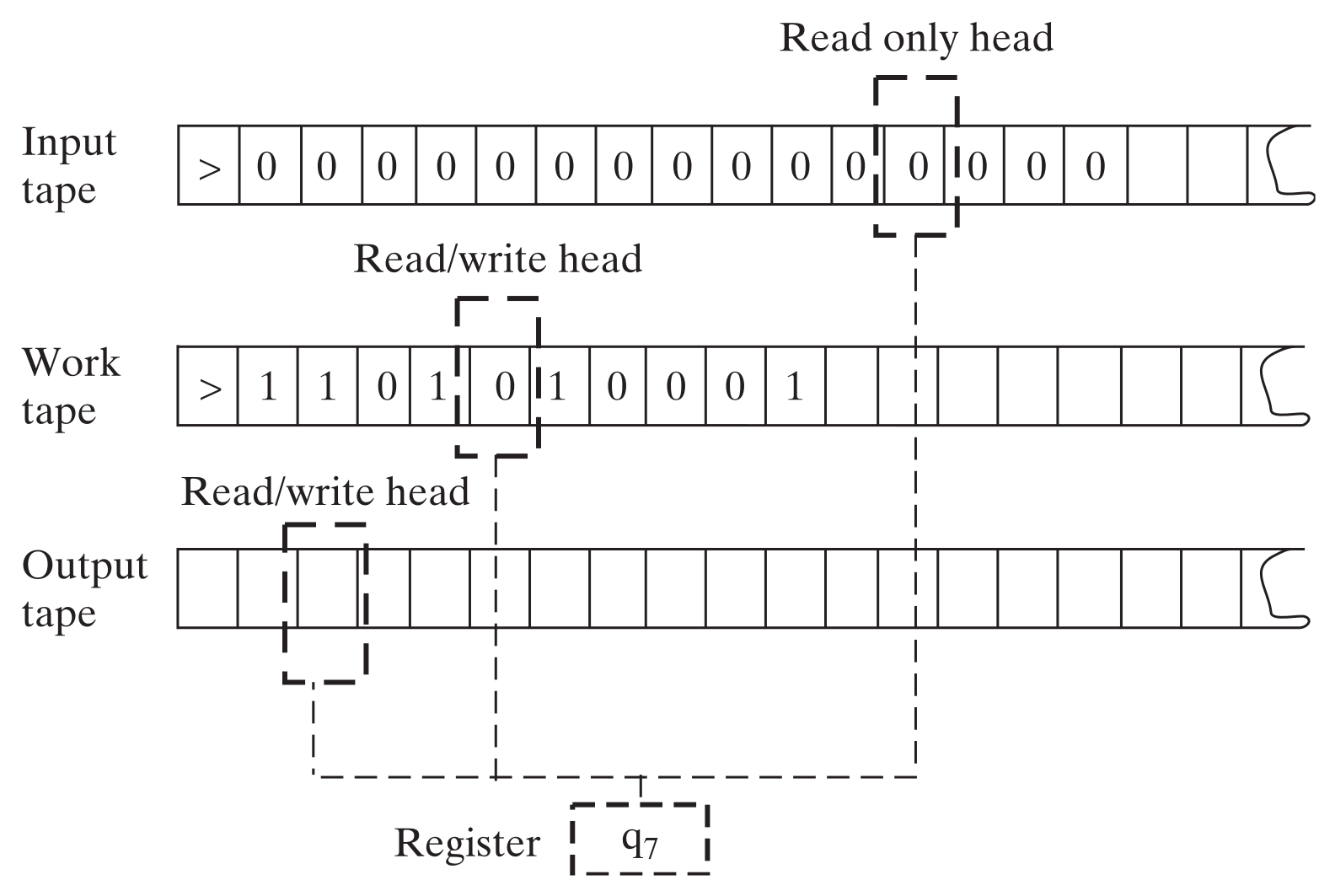
A $k$-tape Turing machine, which we denote by $M$, is a machine with $k$ tapes that are infinitely long in one direction (i.e., they are represented by the set $\mathbb{N}$). The machine $M$ has a single read-only input tape, a single read-write output tape, and $(k-2)$ read-write work tapes. $M$ also contains a register which tracks the machine’s state. Each head can be moved independently. More formally, a $k$-tape Turing machine $M$ is described by a tuple $(\Sigma ,\Gamma ,Q,\delta )$ with the following properties:

1. $\Sigma$ is a finite set, which we call the input alphabet;
2. $\Gamma =\Sigma \cup \{▹,\square \}$ is called the tape alphabet, and it contains $\Sigma$ along with two special symbols that are not in $\Sigma$. $▹\notin \Sigma$ is the start symbol and $\square \notin \Sigma$ is the blank symbol.
3. $Q$ is a finite set of states which can be held in the register. $Q$ always contains two special states: $q_{\mathrm{start}}$ (the start state) and $q_{\mathrm{halt}}$ (the halt state).
4. A transition function $\delta :Q\times {\Gamma }^k\to Q\times {\Gamma }^{k-1}\times \{L,R,S{\}}^k$ describing the rules $M$ follows during a computation.

We say that a tuple $(q,{\gamma }_1,\dots ,{\gamma }_k)\in Q\times {\Gamma }^k$ is a configuration of the Turing machine $M$. In this light, the transition function $\delta$ maps configurations of the Turing machine to new configurations as follows:

• $q$ represents the current state of the machine $M$ stored in its register;
• ${\gamma }_i\in \Gamma$ represents the current symbol under tape $i$’s head, for $i\in [k]$;
• $\delta$ reads the current state and the contents of the $k$ tape heads. It then outputs a new configuration $(q^{\prime },{\gamma }_2^{\prime },\dots ,{\gamma }_k^{\prime },d_1,\dots ,d_k)$, where
  • $q^{\prime }$ is the new state stored in the register;
  • ${\gamma }_i^{\prime }\in \Gamma$ is a new symbol that is written under the $i$th tape head for $i\ge 2$ (i.e., it excludes the input tape); and
  • $d_i\in \{L,R,S\}$ specifies moving tape head $i\in [n]$ one space Left, one space Right, or telling the tape head to Stay.²
• If the Turing machine is ever in the state $q_{mathrmhalt}$, it stops executing the transition function and halts.

Additionally, all Turing machines satisfy the following.

• All $k$ tapes are initially set with $\square$ in every location.
• The first index of every tape is then initialized to $▹$. All tape heads begin here.
• On input $x$, all Turing machines $M$ will:
  • Move the input head $R$, then write $x$ to the input tape.
  • Move the input head $L$ until it reaches $▹$.
  • Set the initial state in the register to $q_{\mathrm{start}}$. The Turing machine is now ready to begin its computation.

We call this the initial configuration of the Turing machine.

A graphical example of a $3$-tape Turing machine is presented below.

Turing machine example: Palindromes

Let’s see an example of a Turing machine in action. We will be using Turing machines to compute functions. Let $f:\{0,1{\}}^{\ast }\to \{0,1\}$ be a function such that $f(x)=1$ if and only if $x\in \{0,1{\}}^{\ast }$ is a palindrome. That is, $x=\mathrm{reverse}(x)$; equivalently, if $n=|x|$, then $x_i=x_{n-i+1}$ for all $i\in [n]$. Let’s design a Turing machine for computing $f$.

High-level TM Specification. Let $M_f$ be a $3$-tape Turing machine (1 input, 1 output, 1 work tape). On input $x\in \{0,1{\}}^n$ for any $n\in \mathbb{N}$, $M_f$ will do the following.

1. Copy the input $x$ to the work tape.

2. Move the input head to the start of the input tape (with $▹$ under the head), leave the work head at the last position (with $\square$ under the head).

3. Move the input head one position right (with $x_1$ under the head) and move the work head one position left (with $x_n$ under the head).

4. Read the symbols under the input head and the work head.

   (a) If the symbol under the input head is $\square$ and the symbol under the work head is $▹$, then write $1$ to the output tape and halt.

   (b) Else if the symbols under the input head and work head are not equal, write $0$ to the output tape and halt.

   (c) Else (i.e., the symbols are equal) move the input head one step right and move the work head one step left.

Formal TM Specification of above. We now formalize thie above process. To do so, we specify (1) the input alphabet; (2) the set of states for $M_f$; and (3) the transition function for $M_f$.

• The input alphabet $\Sigma$ is simply $\{0,1\}$. This tells us our tape alphabet is $\Gamma =\{0,1,▹,\square \}$.
• The set of states will be $Q=\{q_{\mathrm{start}},q_{\mathrm{halt}},q_{\mathrm{copy}},q_{\mathrm{left}},q_{\mathrm{test}}\}$.
• The transition function $\delta :Q\times {\Gamma }^3\to Q\times {\Gamma }^2\times \{L,R,S{\}}^3$ is defined as follows. Let $(q,{\gamma }_1,{\gamma }_2,{\gamma }_3)$ be a configuration given as input to $\delta$.
  • If $q=q_{\mathrm{start}}$, move both the input head and work head right and change the state to $q_{\mathrm{copy}}$.
  • If $q=q_{\mathrm{copy}}$, then read the symbol under the input head (i.e., read ${\gamma }_1$).
    • If ${\gamma }_1\ne \square$, write ${\gamma }_1$ to the current position of the work tape. Then move both the input head and work head one step right. Keep the state as $q_{\mathrm{copy}}$. In this case, the output of the transition function is $(q_{\mathrm{copy}},{\gamma }_1,{\gamma }_3,R,R,S)$.
    • If ${\gamma }_1=\square$, then move the input head left and change the state to $q_{\mathrm{left}}$. In this case, the output of the transition function is $(q_{\mathrm{left}},{\gamma }_2,{\gamma }_3,L,S,S)$.
  • If $q=q_{\mathrm{left}}$, read the symbol under the input head (i.e., ${\gamma }_1$).
    • If ${\gamma }_1\ne ▹$, then move the input head left and keep the state as $q_{\mathrm{left}}$. In this case, the output of the transition function is $(q_{\mathrm{left}},{\gamma }_2,{\gamma }_3,L,S,S)$.
    • If ${\gamma }_1=▹$, then move the input head right, move the work head left, and change the state to $q_{\mathrm{test}}$. In this case, the output of the transition function is $(q_{\mathrm{test}},{\gamma }_2,{\gamma }_3,R,L,S)$.
  • If $q=q_{\mathrm{test}}$, read what’s under the input and work heads (i.e., ${\gamma }_1$ and ${\gamma }_2$).
    • If ${\gamma }_1=\square$ and ${\gamma }_2=▹$, then write $1$ on the output tape and change the state to $q_{\mathrm{halt}}$. In this case, the transition function outputs $(q_{\mathrm{halt}},{\gamma }_2,1,S,S,S)$.
    • Else if ${\gamma }_1\ne {\gamma }_2$, then write $0$ on the output tape and change the state to $q_{\mathrm{halt}}$. In this case, the transition function outputs $(q_{\mathrm{halt}},{\gamma }_2,0,S,S,S)$.
    • Else (i.e., ${\gamma }_1={\gamma }_2$), then move the input head right and the work head left, keeping the state as $q_{\mathrm{test}}$. In this case, the transition function outputs $(q_{\mathrm{test}},{\gamma }_2,{\gamma }_3,R,L,S)$.

Turing Machine Equivalences

At first, the Turing machine model seems like a very restrictive model that cannot compute many things, especially real-life computers. However, as we will see, this restrictive computational model is (roughly) equivalent to nearly every other computational model people have thought of over the years. This includes:

• Random access machines;
• Turing machines with write-only output tapes;
• $\lambda$-calculus;
• Single-tape Turing machines;
• Turing machines with bidirectional infinite tapes;
• Pointer and Counter machines;
• Turing machines with only binary input alphabets;
• Oblivious Turing machines.

In the next lecture or two, we will quantify what we mean by Turing machines being equivalent to the above notions.

1. Quantum computers are the one (almost) physically realizable computational model that we have which does not seem to admit efficient simulation on Turing machines. ↩

2. If the Turing machine specifies that a tape head to move left, but it’s at the start of the tape, the head simply stays in the same place. ↩